贝叶斯高斯混合模型和哈密顿蒙特卡罗

在 TensorFlow.org 上查看

在 Google Colab 中运行

在 GitHub 上查看源代码

下载笔记本

在这个 Colab 中，我们将探索仅使用 TensorFlow Probability 原语从贝叶斯高斯混合模型 (BGMM) 后验中采样。

模型

对于 $k\in\{1,\ldots, K\}$ 个混合分量，每个分量都是 $D$ 维的，我们希望使用以下贝叶斯高斯混合模型对 $i\in\{1,\ldots,N\}$ 个 iid 样本进行建模

$\begin{align*} \theta &\sim \text{Dirichlet}(\text{concentration}=\alpha_0)\\ \mu_k &\sim \text{Normal}(\text{loc}=\mu_{0k}, \text{scale}=I_D)\\ T_k &\sim \text{Wishart}(\text{df}=5, \text{scale}=I_D)\\ Z_i &\sim \text{Categorical}(\text{probs}=\theta)\\ Y_i &\sim \text{Normal}(\text{loc}=\mu_{z_i}, \text{scale}=T_{z_i}^{-1/2})\\ \end{align*}$

注意，scale 参数都具有 cholesky 语义。我们使用此约定，因为它是 TF Distributions 的约定（它本身部分使用此约定，因为它在计算上有利）。

我们的目标是从后验生成样本

$p\left(\theta, \{\mu_k, T_k\}_{k=1}^K \Big| \{y_i\}_{i=1}^N, \alpha_0, \{\mu_{ok}\}_{k=1}^K\right)$

请注意， $\{Z_i\}_{i=1}^N$ 不存在 - 我们只对那些不随 $N$ 缩放的随机变量感兴趣。（幸运的是，有一个 TF 分布可以处理对 $Z_i$ 进行边缘化。）

由于计算上难以处理的归一化项，因此无法直接从该分布中采样。

Metropolis-Hastings 算法是从难以归一化的分布中采样的技术。

TensorFlow Probability 提供了许多 MCMC 选项，包括几个基于 Metropolis-Hastings 的选项。在本笔记本中，我们将使用哈密顿蒙特卡罗 (tfp.mcmc.HamiltonianMonteCarlo)。HMC 通常是一个不错的选择，因为它可以快速收敛，联合采样状态空间（而不是逐坐标采样），并利用 TF 的优势之一：自动微分。也就是说，从 BGMM 后验中采样实际上可能更适合使用其他方法，例如吉布斯采样。

%matplotlib inline


import functools

import matplotlib.pyplot as plt; plt.style.use('ggplot')
import numpy as np
import seaborn as sns; sns.set_context('notebook')

import tensorflow.compat.v2 as tf
tf.enable_v2_behavior()
import tensorflow_probability as tfp

tfd = tfp.distributions
tfb = tfp.bijectors

physical_devices = tf.config.experimental.list_physical_devices('GPU')
if len(physical_devices) > 0:
  tf.config.experimental.set_memory_growth(physical_devices[0], True)

在实际构建模型之前，我们需要定义一种新的分布类型。从上面的模型规范可以清楚地看出，我们使用逆协方差矩阵，即 [精度矩阵](https://en.wikipedia.org/wiki/Precision_(statistics%29) 来参数化 MVN。为了在 TF 中实现这一点，我们需要推出我们的 Bijector。此 Bijector 将使用以下正向变换

Y = tf.linalg.triangular_solve((tf.linalg.matrix_transpose(chol_precision_tril), X, adjoint=True) + loc.

而 log_prob 计算只是反向，即

X = tf.linalg.matmul(chol_precision_tril, X - loc, adjoint_a=True).

由于我们只需要 log_prob，这意味着我们永远不会调用 tf.linalg.triangular_solve（就像 tfd.MultivariateNormalTriL 的情况一样）。这是有利的，因为 tf.linalg.matmul 通常由于更好的缓存局部性而更快。

class MVNCholPrecisionTriL(tfd.TransformedDistribution):
  """MVN from loc and (Cholesky) precision matrix."""

  def __init__(self, loc, chol_precision_tril, name=None):
    super(MVNCholPrecisionTriL, self).__init__(
        distribution=tfd.Independent(tfd.Normal(tf.zeros_like(loc),
                                                scale=tf.ones_like(loc)),
                                     reinterpreted_batch_ndims=1),
        bijector=tfb.Chain([
            tfb.Shift(shift=loc),
            tfb.Invert(tfb.ScaleMatvecTriL(scale_tril=chol_precision_tril,
                                           adjoint=True)),
        ]),
        name=name)

tfd.Independent 分布将一个分布的独立抽取转换为具有统计独立坐标的多元分布。在计算 log_prob 方面，这种“元分布”表现为对事件维度（s）的简单求和。

还要注意，我们对比例矩阵取了 adjoint（“转置”）。这是因为如果精度是逆协方差，即 $P=C^{-1}$ 并且如果 $C=AA^\top$ ，则 $P=BB^{\top}$ ，其中 $B=A^{-\top}$ 。

由于这种分布有点棘手，让我们快速验证一下我们的 MVNCholPrecisionTriL 是否按我们预期的那样工作。

def compute_sample_stats(d, seed=42, n=int(1e6)):
  x = d.sample(n, seed=seed)
  sample_mean = tf.reduce_mean(x, axis=0, keepdims=True)
  s = x - sample_mean
  sample_cov = tf.linalg.matmul(s, s, adjoint_a=True) / tf.cast(n, s.dtype)
  sample_scale = tf.linalg.cholesky(sample_cov)
  sample_mean = sample_mean[0]
  return [
      sample_mean,
      sample_cov,
      sample_scale,
  ]

dtype = np.float32
true_loc = np.array([1., -1.], dtype=dtype)
true_chol_precision = np.array([[1., 0.],
                                [2., 8.]],
                               dtype=dtype)
true_precision = np.matmul(true_chol_precision, true_chol_precision.T)
true_cov = np.linalg.inv(true_precision)

d = MVNCholPrecisionTriL(
    loc=true_loc,
    chol_precision_tril=true_chol_precision)

[sample_mean, sample_cov, sample_scale] = [
    t.numpy() for t in compute_sample_stats(d)]

print('true mean:', true_loc)
print('sample mean:', sample_mean)
print('true cov:\n', true_cov)
print('sample cov:\n', sample_cov)

true mean: [ 1. -1.]
sample mean: [ 1.0002806 -1.000105 ]
true cov:
 [[ 1.0625   -0.03125 ]
 [-0.03125   0.015625]]
sample cov:
 [[ 1.0641273  -0.03126175]
 [-0.03126175  0.01559312]]

由于样本均值和协方差接近真实均值和协方差，因此该分布似乎已正确实现。现在，我们将使用 MVNCholPrecisionTriL tfp.distributions.JointDistributionNamed 来指定 BGMM 模型。对于观测模型，我们将使用 tfd.MixtureSameFamily 来自动积分出 $\{Z_i\}_{i=1}^N$ 抽取。

dtype = np.float64
dims = 2
components = 3
num_samples = 1000

bgmm = tfd.JointDistributionNamed(dict(
  mix_probs=tfd.Dirichlet(
    concentration=np.ones(components, dtype) / 10.),
  loc=tfd.Independent(
    tfd.Normal(
        loc=np.stack([
            -np.ones(dims, dtype),
            np.zeros(dims, dtype),
            np.ones(dims, dtype),
        ]),
        scale=tf.ones([components, dims], dtype)),
    reinterpreted_batch_ndims=2),
  precision=tfd.Independent(
    tfd.WishartTriL(
        df=5,
        scale_tril=np.stack([np.eye(dims, dtype=dtype)]*components),
        input_output_cholesky=True),
    reinterpreted_batch_ndims=1),
  s=lambda mix_probs, loc, precision: tfd.Sample(tfd.MixtureSameFamily(
      mixture_distribution=tfd.Categorical(probs=mix_probs),
      components_distribution=MVNCholPrecisionTriL(
          loc=loc,
          chol_precision_tril=precision)),
      sample_shape=num_samples)
))

def joint_log_prob(observations, mix_probs, loc, chol_precision):
  """BGMM with priors: loc=Normal, precision=Inverse-Wishart, mix=Dirichlet.

  Args:
    observations: `[n, d]`-shaped `Tensor` representing Bayesian Gaussian
      Mixture model draws. Each sample is a length-`d` vector.
    mix_probs: `[K]`-shaped `Tensor` representing random draw from
      `Dirichlet` prior.
    loc: `[K, d]`-shaped `Tensor` representing the location parameter of the
      `K` components.
    chol_precision: `[K, d, d]`-shaped `Tensor` representing `K` lower
      triangular `cholesky(Precision)` matrices, each being sampled from
      a Wishart distribution.

  Returns:
    log_prob: `Tensor` representing joint log-density over all inputs.
  """
  return bgmm.log_prob(
      mix_probs=mix_probs, loc=loc, precision=chol_precision, s=observations)

生成“训练”数据

在本演示中，我们将采样一些随机数据。

true_loc = np.array([[-2., -2],
                     [0, 0],
                     [2, 2]], dtype)
random = np.random.RandomState(seed=43)

true_hidden_component = random.randint(0, components, num_samples)
observations = (true_loc[true_hidden_component] +
                random.randn(num_samples, dims).astype(dtype))

使用 HMC 进行贝叶斯推断

现在我们已经使用 TFD 指定了我们的模型并获得了一些观察数据，我们拥有运行 HMC 所需的所有必要部分。

为此，我们将使用部分应用来“固定”我们不想采样的内容。在这种情况下，这意味着我们只需要固定 observations。（超参数已烘焙到先验分布中，并且不是 joint_log_prob 函数签名的部分。）

unnormalized_posterior_log_prob = functools.partial(joint_log_prob, observations)

initial_state = [
    tf.fill([components],
            value=np.array(1. / components, dtype),
            name='mix_probs'),
    tf.constant(np.array([[-2., -2],
                          [0, 0],
                          [2, 2]], dtype),
                name='loc'),
    tf.linalg.eye(dims, batch_shape=[components], dtype=dtype, name='chol_precision'),
]

无约束表示

哈密顿蒙特卡罗 (HMC) 要求目标对数概率函数对其参数可微。此外，如果状态空间不受约束，HMC 可以表现出显著更高的统计效率。

这意味着在从 BGMM 后验中采样时，我们将需要解决两个主要问题

$\theta$ 表示一个离散概率向量，即必须满足 $\sum_{k=1}^K \theta_k = 1$ 且 $\theta_k>0$ 。
$T_k$ 表示一个逆协方差矩阵，即必须满足 $T_k \succ 0$ ，即为正定。

为了满足此要求，我们需要

将受约束变量转换为无约束空间
在无约束空间中运行 MCMC
将无约束变量转换回受约束空间。

与 MVNCholPrecisionTriL 一样，我们将使用 Bijectors 将随机变量转换为无约束空间。

通过 softmax 函数将 Dirichlet 转换为无约束空间。
我们的精度随机变量是正半定矩阵上的分布。为了取消约束这些矩阵，我们将使用 FillTriangular 和 TransformDiagonal 双射。这些将向量转换为下三角矩阵，并确保对角线为正。前者很有用，因为它允许仅采样 $d(d+1)/2$ 个浮点数，而不是 $d^2$ 个。

unconstraining_bijectors = [
    tfb.SoftmaxCentered(),
    tfb.Identity(),
    tfb.Chain([
        tfb.TransformDiagonal(tfb.Softplus()),
        tfb.FillTriangular(),
    ])]

@tf.function(autograph=False)
def sample():
  return tfp.mcmc.sample_chain(
    num_results=2000,
    num_burnin_steps=500,
    current_state=initial_state,
    kernel=tfp.mcmc.SimpleStepSizeAdaptation(
        tfp.mcmc.TransformedTransitionKernel(
            inner_kernel=tfp.mcmc.HamiltonianMonteCarlo(
                target_log_prob_fn=unnormalized_posterior_log_prob,
                 step_size=0.065,
                 num_leapfrog_steps=5),
            bijector=unconstraining_bijectors),
         num_adaptation_steps=400),
    trace_fn=lambda _, pkr: pkr.inner_results.inner_results.is_accepted)

[mix_probs, loc, chol_precision], is_accepted = sample()

现在我们将执行链并打印后验均值。

acceptance_rate = tf.reduce_mean(tf.cast(is_accepted, dtype=tf.float32)).numpy()
mean_mix_probs = tf.reduce_mean(mix_probs, axis=0).numpy()
mean_loc = tf.reduce_mean(loc, axis=0).numpy()
mean_chol_precision = tf.reduce_mean(chol_precision, axis=0).numpy()
precision = tf.linalg.matmul(chol_precision, chol_precision, transpose_b=True)

print('acceptance_rate:', acceptance_rate)
print('avg mix probs:', mean_mix_probs)
print('avg loc:\n', mean_loc)
print('avg chol(precision):\n', mean_chol_precision)

acceptance_rate: 0.5305
avg mix probs: [0.25248723 0.60729516 0.1402176 ]
avg loc:
 [[-1.96466753 -2.12047249]
 [ 0.27628865  0.22944732]
 [ 2.06461244  2.54216122]]
avg chol(precision):
 [[[ 1.05105032  0.        ]
  [ 0.12699955  1.06553113]]

 [[ 0.76058015  0.        ]
  [-0.50332767  0.77947431]]

 [[ 1.22770457  0.        ]
  [ 0.70670027  1.50914164]]]

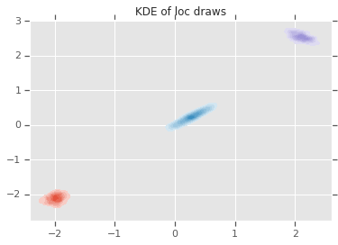
loc_ = loc.numpy()
ax = sns.kdeplot(loc_[:,0,0], loc_[:,0,1], shade=True, shade_lowest=False)
ax = sns.kdeplot(loc_[:,1,0], loc_[:,1,1], shade=True, shade_lowest=False)
ax = sns.kdeplot(loc_[:,2,0], loc_[:,2,1], shade=True, shade_lowest=False)
plt.title('KDE of loc draws');

png

结论

这个简单的 colab 演示了如何使用 TensorFlow Probability 原语来构建分层贝叶斯混合模型。