
 在 TensorFlow.org 上查看 在 TensorFlow.org 上查看
|
 在 Google Colab 中运行 在 Google Colab 中运行
|
 在 GitHub 上查看源代码 在 GitHub 上查看源代码
|
 下载笔记本 下载笔记本
|
本教程介绍了使用 TensorFlow 进行时间序列预测。它构建了几种不同类型的模型,包括卷积神经网络和循环神经网络(CNN 和 RNN)。
这分为两个主要部分,并包含子部分
- 预测单个时间步
- 单个特征。
- 所有特征。
- 预测多个步骤
- 单次预测:一次性进行所有预测。
- 自回归:一次进行一个预测,并将输出反馈给模型。
设置
import os
import datetime

import IPython
import IPython.display
import matplotlib as mpl
import matplotlib.pyplot as plt
import numpy as np
import pandas as pd
import seaborn as sns
import tensorflow as tf

mpl.rcParams['figure.figsize'] = (8, 6)
mpl.rcParams['axes.grid'] = False
2024-06-30 02:52:03.533068: E external/local_xla/xla/stream_executor/cuda/cuda_fft.cc:479] Unable to register cuFFT factory: Attempting to register factory for plugin cuFFT when one has already been registered
2024-06-30 02:52:03.558530: E external/local_xla/xla/stream_executor/cuda/cuda_dnn.cc:10575] Unable to register cuDNN factory: Attempting to register factory for plugin cuDNN when one has already been registered
2024-06-30 02:52:03.558567: E external/local_xla/xla/stream_executor/cuda/cuda_blas.cc:1442] Unable to register cuBLAS factory: Attempting to register factory for plugin cuBLAS when one has already been registered
天气数据集
本教程使用由马克斯·普朗克生物地球化学研究所记录的天气时间序列数据集。
该数据集包含 14 个不同的特征,例如气温、大气压和湿度。这些数据每 10 分钟收集一次,从 2003 年开始。为了提高效率,您将只使用 2009 年至 2016 年间收集的数据。该数据集的这一部分由 François Chollet 为他的著作用 Python 进行深度学习准备。
zip_path = tf.keras.utils.get_file(
    origin='https://storage.googleapis.com/tensorflow/tf-keras-datasets/jena_climate_2009_2016.csv.zip',
    fname='jena_climate_2009_2016.csv.zip',
    extract=True)
csv_path, _ = os.path.splitext(zip_path)
Downloading data from https://storage.googleapis.com/tensorflow/tf-keras-datasets/jena_climate_2009_2016.csv.zip
13568290/13568290 ━━━━━━━━━━━━━━━━━━━━ 0s 0us/step
本教程只处理每小时预测,因此首先从 10 分钟间隔对数据进行二次采样,使其变为每小时间隔。
df = pd.read_csv(csv_path)
# Slice [start:stop:step], starting from index 5 take every 6th record.
df = df[5::6]

date_time = pd.to_datetime(df.pop('Date Time'), format='%d.%m.%Y %H:%M:%S')
让我们看一下数据。以下是前几行。
df.head()
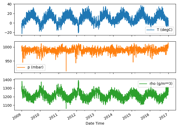
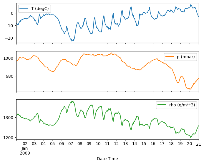
以下是几个特征随时间的演变。
plot_cols = ['T (degC)', 'p (mbar)', 'rho (g/m**3)']
plot_features = df[plot_cols]
plot_features.index = date_time
_ = plot_features.plot(subplots=True)

plot_features = df[plot_cols][:480]
plot_features.index = date_time[:480]
_ = plot_features.plot(subplots=True)
检查和清理
接下来,查看数据集的统计信息。
df.describe().transpose()
风速
应该注意的一点是风速(wv (m/s))列的min值和最大值(max. wv (m/s))列。这个-9999可能是错误的。
有一个单独的风向列,因此风速应该大于零(>=0)。用零替换它。
wv = df['wv (m/s)']
bad_wv = wv == -9999.0
wv[bad_wv] = 0.0

max_wv = df['max. wv (m/s)']
bad_max_wv = max_wv == -9999.0
max_wv[bad_max_wv] = 0.0

# The above inplace edits are reflected in the DataFrame.
df['wv (m/s)'].min()
0.0
特征工程
在深入构建模型之前,了解您的数据并确保将格式正确的数据传递给模型非常重要。
风
数据的最后一列,wd (deg)——给出以度为单位的风向。角度不是好的模型输入:360° 和 0° 应该彼此接近并平滑地环绕。如果风不吹,方向就不重要。
现在,风数据的分布如下所示。
plt.hist2d(df['wd (deg)'], df['wv (m/s)'], bins=(50, 50), vmax=400)
plt.colorbar()
plt.xlabel('Wind Direction [deg]')
plt.ylabel('Wind Velocity [m/s]')
Text(0, 0.5, 'Wind Velocity [m/s]')
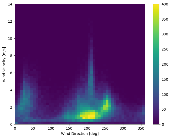
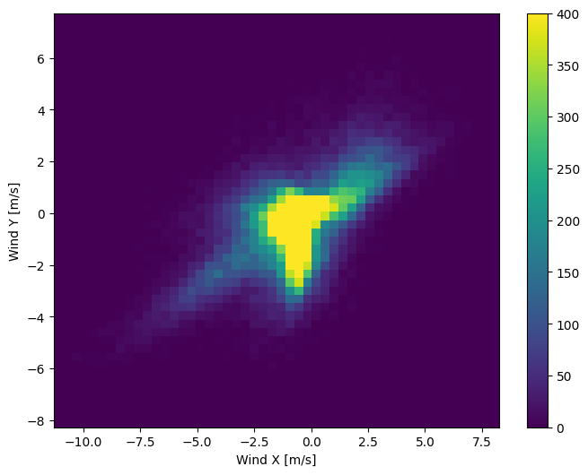
但是,如果您将风向和风速列转换为风向量,模型将更容易解释。
wv = df.pop('wv (m/s)')
max_wv = df.pop('max. wv (m/s)')

# Convert to radians.
wd_rad = df.pop('wd (deg)')*np.pi / 180

# Calculate the wind x and y components.
df['Wx'] = wv*np.cos(wd_rad)
df['Wy'] = wv*np.sin(wd_rad)

# Calculate the max wind x and y components.
df['max Wx'] = max_wv*np.cos(wd_rad)
df['max Wy'] = max_wv*np.sin(wd_rad)
风向量的分布对于模型正确解释来说要简单得多。
plt.hist2d(df['Wx'], df['Wy'], bins=(50, 50), vmax=400)
plt.colorbar()
plt.xlabel('Wind X [m/s]')
plt.ylabel('Wind Y [m/s]')
ax = plt.gca()
ax.axis('tight')
(-11.305513973134667, 8.24469928549079, -8.27438540335515, 7.7338312955467785)
时间
类似地,Date Time列非常有用,但不是这种字符串形式。首先将其转换为秒。
timestamp_s = date_time.map(pd.Timestamp.timestamp)
与风向类似,以秒为单位的时间不是有用的模型输入。作为天气数据,它具有明显的每日和每年周期性。您可以用多种方法处理周期性。
您可以使用正弦和余弦变换来获取可用的信号,以清除“一天中的时间”和“一年中的时间”信号。
day = 24*60*60
year = (365.2425)*day

df['Day sin'] = np.sin(timestamp_s * (2 * np.pi / day))
df['Day cos'] = np.cos(timestamp_s * (2 * np.pi / day))
df['Year sin'] = np.sin(timestamp_s * (2 * np.pi / year))
df['Year cos'] = np.cos(timestamp_s * (2 * np.pi / year))
plt.plot(np.array(df['Day sin'])[:25])
plt.plot(np.array(df['Day cos'])[:25])
plt.xlabel('Time [h]')
plt.title('Time of day signal')
Text(0.5, 1.0, 'Time of day signal')
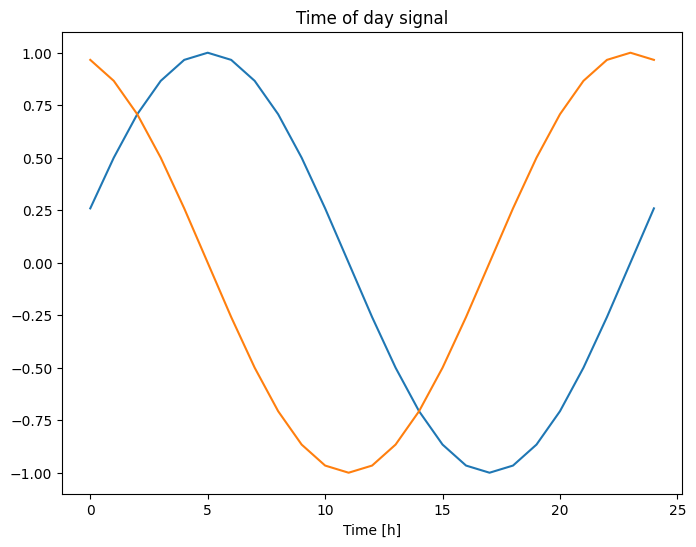
这使模型能够访问最重要的频率特征。在这种情况下,您事先知道哪些频率很重要。
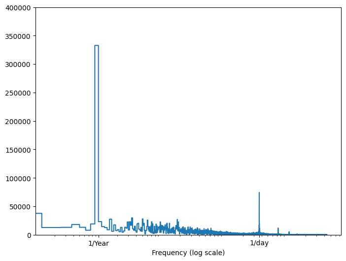
如果您没有这些信息,可以使用快速傅里叶变换提取特征来确定哪些频率很重要。为了验证假设,以下是温度随时间的tf.signal.rfft。注意在接近1/year和1/day的频率处明显的峰值。
fft = tf.signal.rfft(df['T (degC)'])
f_per_dataset = np.arange(0, len(fft))

n_samples_h = len(df['T (degC)'])
hours_per_year = 24*365.2524
years_per_dataset = n_samples_h/(hours_per_year)

f_per_year = f_per_dataset/years_per_dataset
plt.step(f_per_year, np.abs(fft))
plt.xscale('log')
plt.ylim(0, 400000)
plt.xlim([0.1, max(plt.xlim())])
plt.xticks([1, 365.2524], labels=['1/Year', '1/day'])
_ = plt.xlabel('Frequency (log scale)')
拆分数据
您将使用(70%, 20%, 10%)的拆分来进行训练、验证和测试集。请注意,数据没有在拆分之前随机洗牌。这是出于两个原因。
- 它确保将数据切分成连续样本的窗口仍然是可能的。
- 它确保验证/测试结果更现实,因为它们是在模型训练后收集的数据上进行评估的。
column_indices = {name: i for i, name in enumerate(df.columns)}

n = len(df)
train_df = df[0:int(n*0.7)]
val_df = df[int(n*0.7):int(n*0.9)]
test_df = df[int(n*0.9):]

num_features = df.shape[1]
规范化数据
在训练神经网络之前对特征进行缩放非常重要。规范化是一种常见的缩放方法:减去每个特征的均值并除以标准差。
均值和标准差应该只使用训练数据计算,这样模型就无法访问验证集和测试集中的值。
也可以说,模型在训练时不应该访问训练集中未来的值,并且这种规范化应该使用移动平均值进行。这不是本教程的重点,验证集和测试集确保您获得(某种程度上)诚实的指标。因此,为了简单起见,本教程使用简单的平均值。
train_mean = train_df.mean()
train_std = train_df.std()

train_df = (train_df - train_mean) / train_std
val_df = (val_df - train_mean) / train_std
test_df = (test_df - train_mean) / train_std
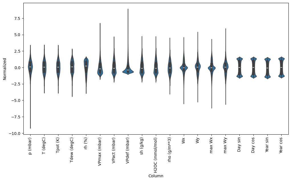
现在,看一下特征的分布。一些特征确实有长尾,但没有像-9999风速值那样明显的错误。
df_std = (df - train_mean) / train_std
df_std = df_std.melt(var_name='Column', value_name='Normalized')
plt.figure(figsize=(12, 6))
ax = sns.violinplot(x='Column', y='Normalized', data=df_std)
_ = ax.set_xticklabels(df.keys(), rotation=90)
/tmpfs/tmp/ipykernel_117798/3214313372.py:5: UserWarning: set_ticklabels() should only be used with a fixed number of ticks, i.e. after set_ticks() or using a FixedLocator.
  _ = ax.set_xticklabels(df.keys(), rotation=90)
数据窗口
本教程中的模型将根据数据中一组连续样本的窗口进行一组预测。
输入窗口的主要特征是
- 输入和标签窗口的宽度(时间步数)。
- 它们之间的时间偏移。
- 哪些特征用作输入、标签或两者。
本教程构建了各种模型(包括线性模型、DNN 模型、CNN 模型和 RNN 模型),并将其用于以下两种情况。
- 单输出和多输出预测。
- 单时间步和多时间步预测。
本节重点介绍数据窗口的实现,以便可以将其重复用于所有这些模型。
根据任务和模型类型,您可能希望生成各种数据窗口。以下是一些示例。
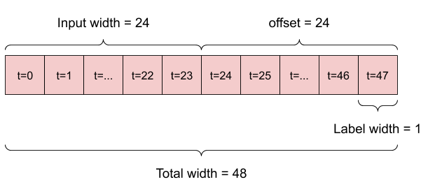
例如,要根据 24 小时的历史记录预测未来 24 小时的单一预测,您可以这样定义窗口。
一个根据 6 小时的历史记录预测未来 1 小时的模型,需要这样的窗口。
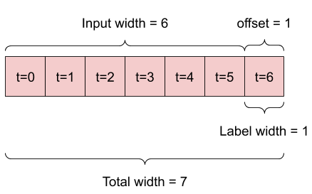
本节的其余部分定义了一个WindowGenerator类。此类可以
- 处理上面图表中显示的索引和偏移量。
- 将特征窗口拆分为
(features, labels)对。 - 绘制生成的窗口的内容。
- 使用
tf.data.Dataset从训练、评估和测试数据中有效地生成这些窗口的批次。
1. 索引和偏移量
首先创建WindowGenerator类。该__init__方法包含输入和标签索引所需的所有逻辑。
它还将训练、评估和测试 DataFrame 作为输入。这些将在稍后转换为tf.data.Dataset的窗口。
class WindowGenerator():
  def __init__(self, input_width, label_width, shift,
               train_df=train_df, val_df=val_df, test_df=test_df,
               label_columns=None):
    # Store the raw data.
    self.train_df = train_df
    self.val_df = val_df
    self.test_df = test_df

    # Work out the label column indices.
    self.label_columns = label_columns
    if label_columns is not None:
      self.label_columns_indices = {name: i for i, name in
                                    enumerate(label_columns)}
    self.column_indices = {name: i for i, name in
                           enumerate(train_df.columns)}

    # Work out the window parameters.
    self.input_width = input_width
    self.label_width = label_width
    self.shift = shift

    self.total_window_size = input_width + shift

    self.input_slice = slice(0, input_width)
    self.input_indices = np.arange(self.total_window_size)[self.input_slice]

    self.label_start = self.total_window_size - self.label_width
    self.labels_slice = slice(self.label_start, None)
    self.label_indices = np.arange(self.total_window_size)[self.labels_slice]

  def __repr__(self):
    return '\n'.join([
        f'Total window size: {self.total_window_size}',
        f'Input indices: {self.input_indices}',
        f'Label indices: {self.label_indices}',
        f'Label column name(s): {self.label_columns}'])
以下代码用于创建本节开头图表中显示的两个窗口。
w1 = WindowGenerator(input_width=24, label_width=1, shift=24,
                     label_columns=['T (degC)'])
w1
Total window size: 48
Input indices: [ 0  1  2  3  4  5  6  7  8  9 10 11 12 13 14 15 16 17 18 19 20 21 22 23]
Label indices: [47]
Label column name(s): ['T (degC)']
w2 = WindowGenerator(input_width=6, label_width=1, shift=1,
                     label_columns=['T (degC)'])
w2
Total window size: 7
Input indices: [0 1 2 3 4 5]
Label indices: [6]
Label column name(s): ['T (degC)']
2. 拆分
给定一系列连续的输入,split_window方法将它们转换为一个输入窗口和一个标签窗口。
您之前定义的示例w2将这样拆分。
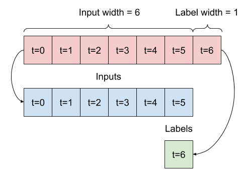
此图表没有显示数据的features轴,但此split_window函数还处理label_columns,因此它可以用于单输出和多输出示例。
def split_window(self, features):
  inputs = features[:, self.input_slice, :]
  labels = features[:, self.labels_slice, :]
  if self.label_columns is not None:
    labels = tf.stack(
        [labels[:, :, self.column_indices[name]] for name in self.label_columns],
        axis=-1)

  # Slicing doesn't preserve static shape information, so set the shapes
  # manually. This way the `tf.data.Datasets` are easier to inspect.
  inputs.set_shape([None, self.input_width, None])
  labels.set_shape([None, self.label_width, None])

  return inputs, labels

WindowGenerator.split_window = split_window
试一试
# Stack three slices, the length of the total window.
example_window = tf.stack([np.array(train_df[:w2.total_window_size]),
                           np.array(train_df[100:100+w2.total_window_size]),
                           np.array(train_df[200:200+w2.total_window_size])])

example_inputs, example_labels = w2.split_window(example_window)

print('All shapes are: (batch, time, features)')
print(f'Window shape: {example_window.shape}')
print(f'Inputs shape: {example_inputs.shape}')
print(f'Labels shape: {example_labels.shape}')
All shapes are: (batch, time, features)
Window shape: (3, 7, 19)
Inputs shape: (3, 6, 19)
Labels shape: (3, 1, 1)
通常,TensorFlow 中的数据被打包成数组,其中最外层的索引是跨示例(“批次”维度)。中间索引是“时间”或“空间”(宽度、高度)维度。最内层的索引是特征。
上面的代码获取了三个 7 时间步窗口的批次,每个时间步有 19 个特征。它将它们拆分为 6 时间步 19 特征输入的批次和 1 时间步 1 特征标签。标签只有一个特征,因为WindowGenerator是用label_columns=['T (degC)']初始化的。最初,本教程将构建预测单输出标签的模型。
3. 绘制
以下是一个绘制方法,它允许简单地可视化拆分的窗口。
w2.example = example_inputs, example_labels
def plot(self, model=None, plot_col='T (degC)', max_subplots=3):
  inputs, labels = self.example
  plt.figure(figsize=(12, 8))
  plot_col_index = self.column_indices[plot_col]
  max_n = min(max_subplots, len(inputs))
  for n in range(max_n):
    plt.subplot(max_n, 1, n+1)
    plt.ylabel(f'{plot_col} [normed]')
    plt.plot(self.input_indices, inputs[n, :, plot_col_index],
             label='Inputs', marker='.', zorder=-10)

    if self.label_columns:
      label_col_index = self.label_columns_indices.get(plot_col, None)
    else:
      label_col_index = plot_col_index

    if label_col_index is None:
      continue

    plt.scatter(self.label_indices, labels[n, :, label_col_index],
                edgecolors='k', label='Labels', c='#2ca02c', s=64)
    if model is not None:
      predictions = model(inputs)
      plt.scatter(self.label_indices, predictions[n, :, label_col_index],
                  marker='X', edgecolors='k', label='Predictions',
                  c='#ff7f0e', s=64)

    if n == 0:
      plt.legend()

  plt.xlabel('Time [h]')

WindowGenerator.plot = plot
此图根据项目所指的时间对输入、标签和(稍后)预测进行对齐。
w2.plot()
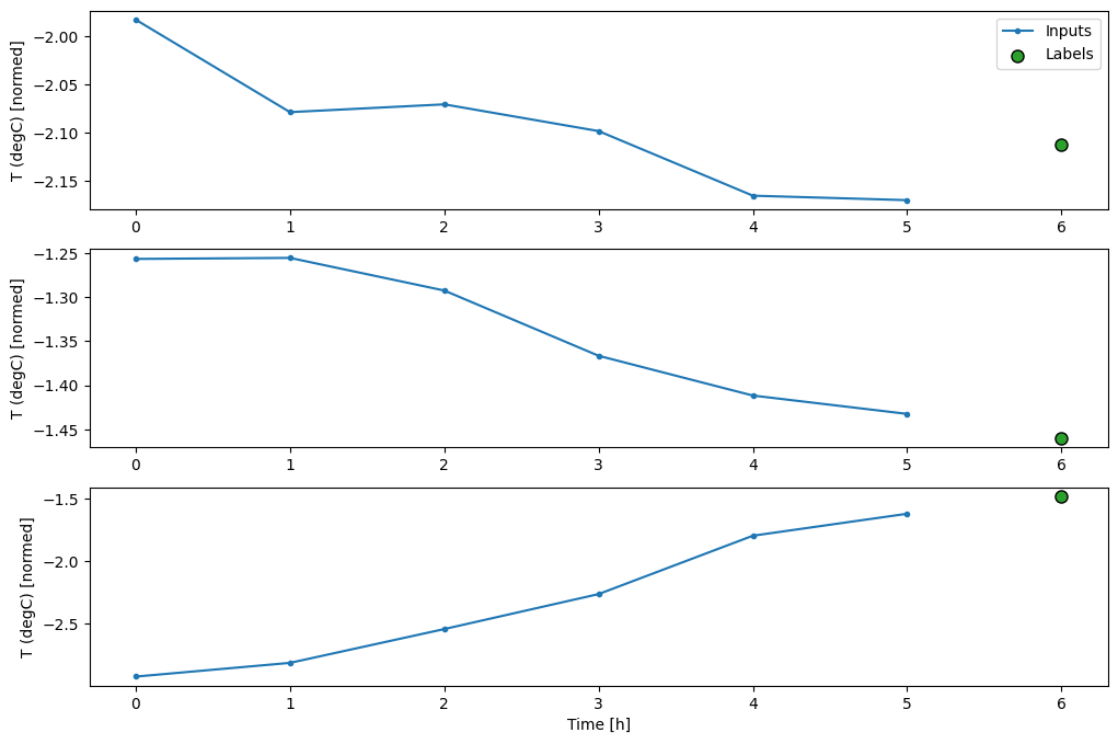
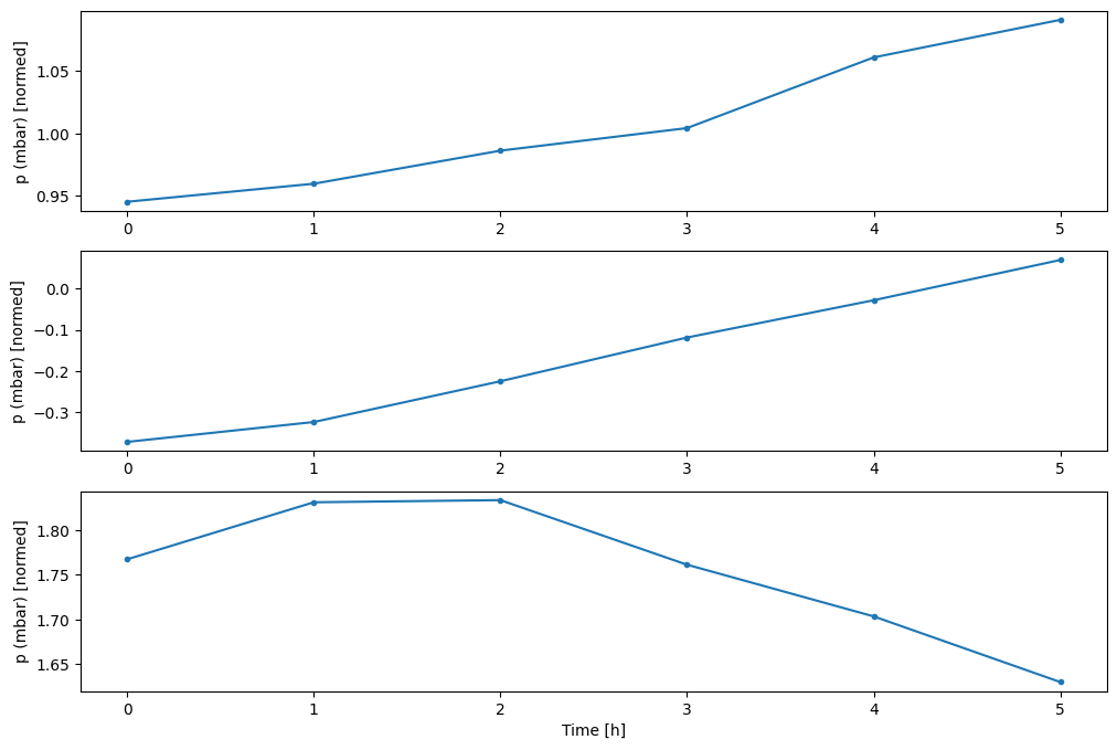
您可以绘制其他列,但示例窗口w2配置只对T (degC)列有标签。
w2.plot(plot_col='p (mbar)')
4. 创建tf.data.Datasets
最后,此make_dataset方法将获取时间序列 DataFrame 并将其转换为tf.data.Dataset的(input_window, label_window)对,使用tf.keras.utils.timeseries_dataset_from_array函数。
def make_dataset(self, data):
  data = np.array(data, dtype=np.float32)
  ds = tf.keras.utils.timeseries_dataset_from_array(
      data=data,
      targets=None,
      sequence_length=self.total_window_size,
      sequence_stride=1,
      shuffle=True,
      batch_size=32,)

  ds = ds.map(self.split_window)

  return ds

WindowGenerator.make_dataset = make_dataset
该WindowGenerator对象包含训练、验证和测试数据。
添加属性,以便使用之前定义的make_dataset方法将它们作为tf.data.Dataset进行访问。此外,添加一个标准示例批次,以便于访问和绘制。
@property
def train(self):
  return self.make_dataset(self.train_df)

@property
def val(self):
  return self.make_dataset(self.val_df)

@property
def test(self):
  return self.make_dataset(self.test_df)

@property
def example(self):
  """Get and cache an example batch of `inputs, labels` for plotting."""
  result = getattr(self, '_example', None)
  if result is None:
    # No example batch was found, so get one from the `.train` dataset
    result = next(iter(self.train))
    # And cache it for next time
    self._example = result
  return result

WindowGenerator.train = train
WindowGenerator.val = val
WindowGenerator.test = test
WindowGenerator.example = example
现在,WindowGenerator对象使您可以访问tf.data.Dataset对象,因此您可以轻松地遍历数据。
该Dataset.element_spec属性告诉您数据集元素的结构、数据类型和形状。
# Each element is an (inputs, label) pair.
w2.train.element_spec
(TensorSpec(shape=(None, 6, 19), dtype=tf.float32, name=None),
 TensorSpec(shape=(None, 1, 1), dtype=tf.float32, name=None))
遍历Dataset会产生具体的批次。
for example_inputs, example_labels in w2.train.take(1):
  print(f'Inputs shape (batch, time, features): {example_inputs.shape}')
  print(f'Labels shape (batch, time, features): {example_labels.shape}')
Inputs shape (batch, time, features): (32, 6, 19)
Labels shape (batch, time, features): (32, 1, 1)
2024-06-30 02:52:21.131505: W tensorflow/core/framework/local_rendezvous.cc:404] Local rendezvous is aborting with status: OUT_OF_RANGE: End of sequence
单步模型
您可以在此类数据上构建的最简单的模型是预测单个特征的值——基于当前条件预测未来 1 个时间步(1 小时)。
因此,首先构建模型来预测未来 1 小时的T (degC)值。
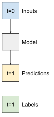
配置一个WindowGenerator对象来生成这些单步(input, label)对。
single_step_window = WindowGenerator(
    input_width=1, label_width=1, shift=1,
    label_columns=['T (degC)'])
single_step_window
Total window size: 2
Input indices: [0]
Label indices: [1]
Label column name(s): ['T (degC)']
该window对象从训练、验证和测试集中创建tf.data.Datasets,使您可以轻松地遍历数据的批次。
for example_inputs, example_labels in single_step_window.train.take(1):
  print(f'Inputs shape (batch, time, features): {example_inputs.shape}')
  print(f'Labels shape (batch, time, features): {example_labels.shape}')
Inputs shape (batch, time, features): (32, 1, 19)
Labels shape (batch, time, features): (32, 1, 1)
2024-06-30 02:52:21.281467: W tensorflow/core/framework/local_rendezvous.cc:404] Local rendezvous is aborting with status: OUT_OF_RANGE: End of sequence
基线
在构建可训练模型之前,最好有一个性能基线作为与以后更复杂的模型进行比较的参考点。
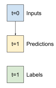
第一个任务是根据所有特征的当前值预测未来 1 小时的温度。当前值包括当前温度。
因此,首先使用一个模型,该模型只返回当前温度作为预测,预测“无变化”。这是一个合理的基线,因为温度变化缓慢。当然,如果您预测更远的未来,此基线的效果会更差。
class Baseline(tf.keras.Model):
  def __init__(self, label_index=None):
    super().__init__()
    self.label_index = label_index

  def call(self, inputs):
    if self.label_index is None:
      return inputs
    result = inputs[:, :, self.label_index]
    return result[:, :, tf.newaxis]
实例化并评估此模型。
baseline = Baseline(label_index=column_indices['T (degC)'])

baseline.compile(loss=tf.keras.losses.MeanSquaredError(),
                 metrics=[tf.keras.metrics.MeanAbsoluteError()])

val_performance = {}
performance = {}
val_performance['Baseline'] = baseline.evaluate(single_step_window.val, return_dict=True)
performance['Baseline'] = baseline.evaluate(single_step_window.test, verbose=0, return_dict=True)
1/439 ━━━━━━━━━━━━━━━━━━━━ 2:24 330ms/step - loss: 0.0173 - mean_absolute_error: 0.0970
WARNING: All log messages before absl::InitializeLog() is called are written to STDERR
I0000 00:00:1719715941.527831  117969 service.cc:145] XLA service 0x7f1550004690 initialized for platform CUDA (this does not guarantee that XLA will be used). Devices:
I0000 00:00:1719715941.527904  117969 service.cc:153]   StreamExecutor device (0): Tesla T4, Compute Capability 7.5
I0000 00:00:1719715941.527913  117969 service.cc:153]   StreamExecutor device (1): Tesla T4, Compute Capability 7.5
I0000 00:00:1719715941.527919  117969 service.cc:153]   StreamExecutor device (2): Tesla T4, Compute Capability 7.5
I0000 00:00:1719715941.527925  117969 service.cc:153]   StreamExecutor device (3): Tesla T4, Compute Capability 7.5
I0000 00:00:1719715941.694380  117969 device_compiler.h:188] Compiled cluster using XLA!  This line is logged at most once for the lifetime of the process.
439/439 ━━━━━━━━━━━━━━━━━━━━ 1s 1ms/step - loss: 0.0126 - mean_absolute_error: 0.0782
这将打印一些性能指标,但这些指标并不能让您了解模型的运行情况。
该WindowGenerator有一个绘制方法,但如果只有一个样本,这些图将不会很有趣。
因此,创建一个更宽的 WindowGenerator,它一次生成 24 小时连续输入和标签的窗口。新的 wide_window 变量不会改变模型的操作方式。模型仍然根据单个输入时间步长预测未来一小时。在这里,time 轴充当 batch 轴:每个预测都是独立进行的,时间步长之间没有交互。
wide_window = WindowGenerator(
    input_width=24, label_width=24, shift=1,
    label_columns=['T (degC)'])

wide_window
Total window size: 25
Input indices: [ 0  1  2  3  4  5  6  7  8  9 10 11 12 13 14 15 16 17 18 19 20 21 22 23]
Label indices: [ 1  2  3  4  5  6  7  8  9 10 11 12 13 14 15 16 17 18 19 20 21 22 23 24]
Label column name(s): ['T (degC)']
这个扩展的窗口可以直接传递给相同的 baseline 模型,无需任何代码更改。这是因为输入和标签具有相同数量的时间步长,而基线模型只是将输入转发到输出。
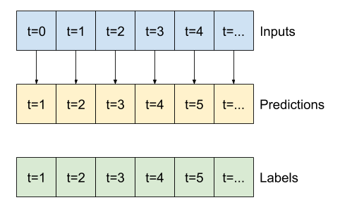
print('Input shape:', wide_window.example[0].shape)
print('Output shape:', baseline(wide_window.example[0]).shape)
Input shape: (32, 24, 19)
Output shape: (32, 24, 1)
通过绘制基线模型的预测,可以注意到它只是将标签向右移动了一小时。
wide_window.plot(baseline)
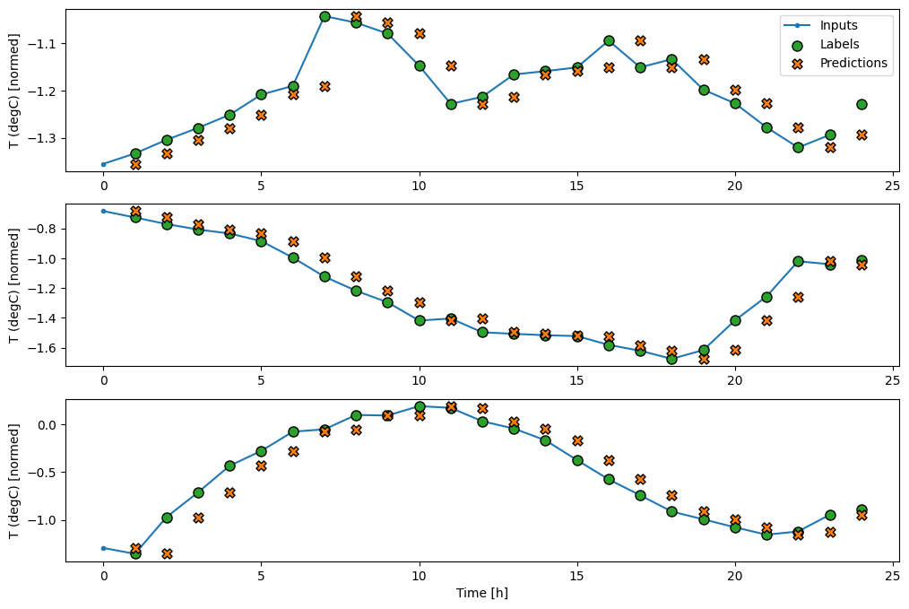
在上面三个示例的图中,单步模型在 24 小时内运行。这需要一些解释。
- 蓝色的
Inputs线显示每个时间步长的输入温度。模型接收所有特征,此图仅显示温度。 - 绿色的
Labels点显示目标预测值。这些点显示在预测时间,而不是输入时间。这就是为什么标签的范围相对于输入移动了 1 步。 - 橙色的
Predictions十字表示模型对每个输出时间步长的预测。如果模型预测完美,预测将直接落在Labels上。
线性模型
您可以应用于此任务的最简单的可训练模型是在输入和输出之间插入线性变换。在这种情况下,时间步长的输出仅取决于该步长。
一个没有设置 activation 的 tf.keras.layers.Dense 层是一个线性模型。该层仅将数据的最后一个轴从 (batch, time, inputs) 变换为 (batch, time, units);它独立地应用于 batch 和 time 轴上的每个项目。
linear = tf.keras.Sequential([
    tf.keras.layers.Dense(units=1)
])
print('Input shape:', single_step_window.example[0].shape)
print('Output shape:', linear(single_step_window.example[0]).shape)
Input shape: (32, 1, 19)
Output shape: (32, 1, 1)
本教程训练了许多模型,因此将训练过程打包到一个函数中。
MAX_EPOCHS = 20

def compile_and_fit(model, window, patience=2):
  early_stopping = tf.keras.callbacks.EarlyStopping(monitor='val_loss',
                                                    patience=patience,
                                                    mode='min')

  model.compile(loss=tf.keras.losses.MeanSquaredError(),
                optimizer=tf.keras.optimizers.Adam(),
                metrics=[tf.keras.metrics.MeanAbsoluteError()])

  history = model.fit(window.train, epochs=MAX_EPOCHS,
                      validation_data=window.val,
                      callbacks=[early_stopping])
  return history
训练模型并评估其性能。
history = compile_and_fit(linear, single_step_window)

val_performance['Linear'] = linear.evaluate(single_step_window.val, return_dict=True)
performance['Linear'] = linear.evaluate(single_step_window.test, verbose=0, return_dict=True)
Epoch 1/20
1534/1534 ━━━━━━━━━━━━━━━━━━━━ 4s 2ms/step - loss: 0.2368 - mean_absolute_error: 0.3324 - val_loss: 0.0157 - val_mean_absolute_error: 0.0936
Epoch 2/20
1534/1534 ━━━━━━━━━━━━━━━━━━━━ 2s 2ms/step - loss: 0.0134 - mean_absolute_error: 0.0870 - val_loss: 0.0109 - val_mean_absolute_error: 0.0790
Epoch 3/20
1534/1534 ━━━━━━━━━━━━━━━━━━━━ 2s 2ms/step - loss: 0.0100 - mean_absolute_error: 0.0741 - val_loss: 0.0091 - val_mean_absolute_error: 0.0713
Epoch 4/20
1534/1534 ━━━━━━━━━━━━━━━━━━━━ 2s 2ms/step - loss: 0.0091 - mean_absolute_error: 0.0699 - val_loss: 0.0089 - val_mean_absolute_error: 0.0701
Epoch 5/20
1534/1534 ━━━━━━━━━━━━━━━━━━━━ 2s 2ms/step - loss: 0.0090 - mean_absolute_error: 0.0695 - val_loss: 0.0088 - val_mean_absolute_error: 0.0699
Epoch 6/20
1534/1534 ━━━━━━━━━━━━━━━━━━━━ 2s 2ms/step - loss: 0.0090 - mean_absolute_error: 0.0695 - val_loss: 0.0088 - val_mean_absolute_error: 0.0696
Epoch 7/20
1534/1534 ━━━━━━━━━━━━━━━━━━━━ 2s 2ms/step - loss: 0.0090 - mean_absolute_error: 0.0693 - val_loss: 0.0089 - val_mean_absolute_error: 0.0701
Epoch 8/20
1534/1534 ━━━━━━━━━━━━━━━━━━━━ 2s 2ms/step - loss: 0.0089 - mean_absolute_error: 0.0693 - val_loss: 0.0088 - val_mean_absolute_error: 0.0698
439/439 ━━━━━━━━━━━━━━━━━━━━ 1s 1ms/step - loss: 0.0088 - mean_absolute_error: 0.0697
与 baseline 模型一样,线性模型可以在宽窗口批次上调用。以这种方式使用,模型对连续时间步长进行一组独立预测。 time 轴充当另一个 batch 轴。每个时间步长的预测之间没有交互。
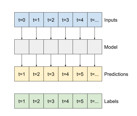
print('Input shape:', wide_window.example[0].shape)
print('Output shape:', linear(wide_window.example[0]).shape)
Input shape: (32, 24, 19)
Output shape: (32, 24, 1)
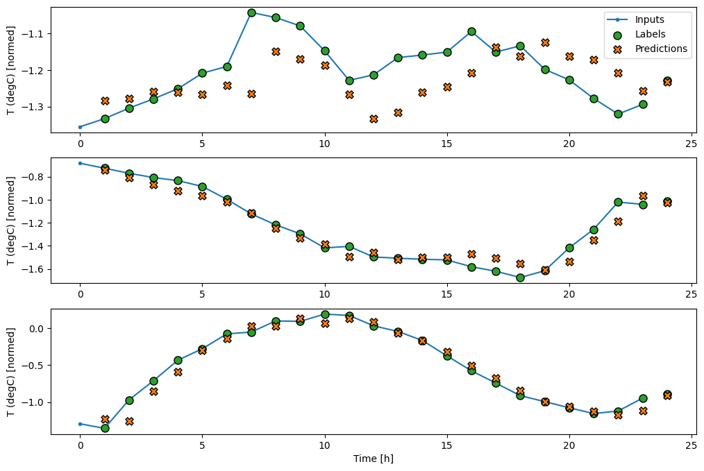
这是它在 wide_window 上的示例预测图,请注意,在许多情况下,预测明显优于仅返回输入温度,但在少数情况下,它更差。
wide_window.plot(linear)
线性模型的一个优点是它们相对容易解释。您可以提取层的权重并可视化分配给每个输入的权重。
plt.bar(x = range(len(train_df.columns)),
        height=linear.layers[0].kernel[:,0].numpy())
axis = plt.gca()
axis.set_xticks(range(len(train_df.columns)))
_ = axis.set_xticklabels(train_df.columns, rotation=90)
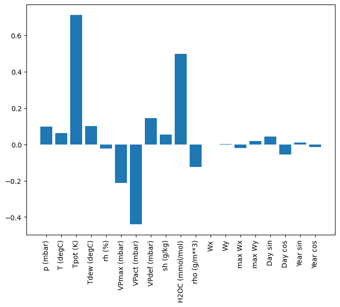
有时模型甚至不会将最大的权重放在输入 T (degC) 上。这是随机初始化的风险之一。
Dense
在应用实际操作多个时间步长的模型之前,值得检查更深、更强大、单输入步长模型的性能。
这是一个类似于 linear 模型的模型,只是它在输入和输出之间堆叠了几个 Dense 层。
dense = tf.keras.Sequential([
    tf.keras.layers.Dense(units=64, activation='relu'),
    tf.keras.layers.Dense(units=64, activation='relu'),
    tf.keras.layers.Dense(units=1)
])

history = compile_and_fit(dense, single_step_window)

val_performance['Dense'] = dense.evaluate(single_step_window.val, return_dict=True)
performance['Dense'] = dense.evaluate(single_step_window.test, verbose=0, return_dict=True)
Epoch 1/20
1534/1534 ━━━━━━━━━━━━━━━━━━━━ 5s 2ms/step - loss: 0.0621 - mean_absolute_error: 0.1284 - val_loss: 0.0086 - val_mean_absolute_error: 0.0676
Epoch 2/20
1534/1534 ━━━━━━━━━━━━━━━━━━━━ 3s 2ms/step - loss: 0.0082 - mean_absolute_error: 0.0659 - val_loss: 0.0071 - val_mean_absolute_error: 0.0605
Epoch 3/20
1534/1534 ━━━━━━━━━━━━━━━━━━━━ 3s 2ms/step - loss: 0.0076 - mean_absolute_error: 0.0631 - val_loss: 0.0070 - val_mean_absolute_error: 0.0591
Epoch 4/20
1534/1534 ━━━━━━━━━━━━━━━━━━━━ 3s 2ms/step - loss: 0.0074 - mean_absolute_error: 0.0615 - val_loss: 0.0066 - val_mean_absolute_error: 0.0574
Epoch 5/20
1534/1534 ━━━━━━━━━━━━━━━━━━━━ 3s 2ms/step - loss: 0.0071 - mean_absolute_error: 0.0602 - val_loss: 0.0067 - val_mean_absolute_error: 0.0579
Epoch 6/20
1534/1534 ━━━━━━━━━━━━━━━━━━━━ 3s 2ms/step - loss: 0.0071 - mean_absolute_error: 0.0603 - val_loss: 0.0069 - val_mean_absolute_error: 0.0593
439/439 ━━━━━━━━━━━━━━━━━━━━ 1s 1ms/step - loss: 0.0072 - mean_absolute_error: 0.0601
多步密集
单时间步长模型没有其输入当前值的上下文。它无法看到输入特征如何随时间变化。为了解决这个问题,模型需要在进行预测时访问多个时间步长。
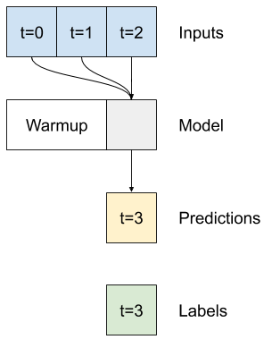
baseline、linear 和 dense 模型独立处理每个时间步长。在这里,模型将以多个时间步长作为输入来生成单个输出。
创建一个 WindowGenerator,它将生成三小时输入和一小时标签的批次。
请注意,Window 的 shift 参数相对于两个窗口的末尾。
CONV_WIDTH = 3
conv_window = WindowGenerator(
    input_width=CONV_WIDTH,
    label_width=1,
    shift=1,
    label_columns=['T (degC)'])

conv_window
Total window size: 4
Input indices: [0 1 2]
Label indices: [3]
Label column name(s): ['T (degC)']
conv_window.plot()
plt.suptitle("Given 3 hours of inputs, predict 1 hour into the future.")
Text(0.5, 0.98, 'Given 3 hours of inputs, predict 1 hour into the future.')
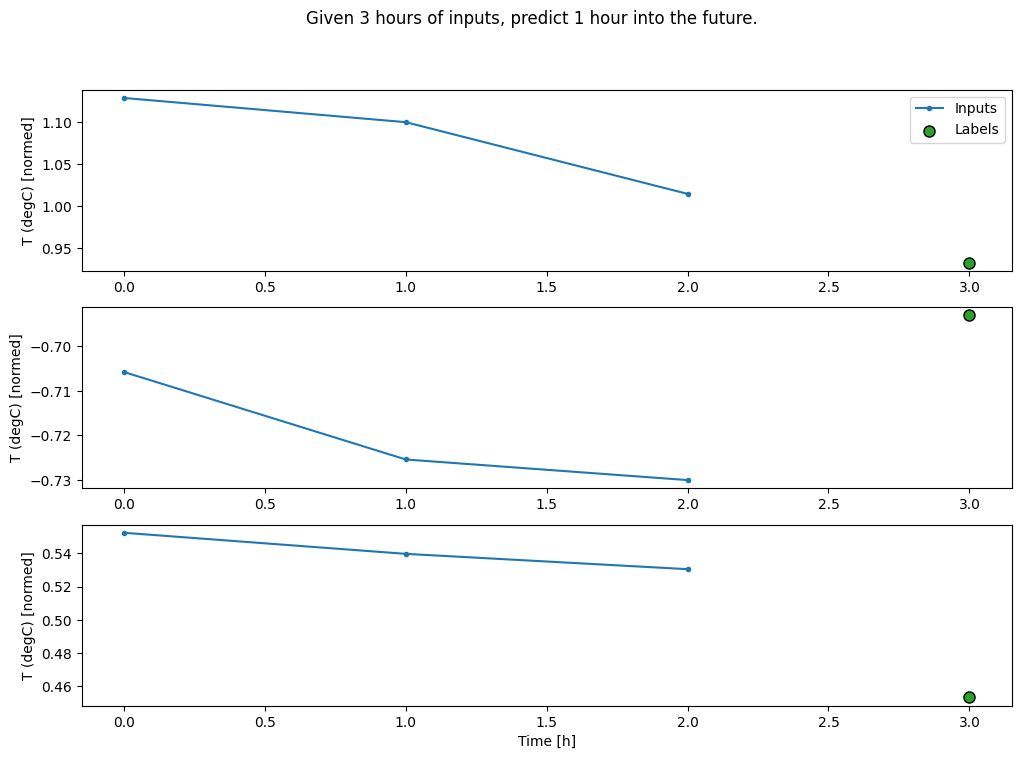
您可以通过在模型的第一层添加 tf.keras.layers.Flatten 来在多输入步长窗口上训练 dense 模型。
multi_step_dense = tf.keras.Sequential([
    # Shape: (time, features) => (time*features)
    tf.keras.layers.Flatten(),
    tf.keras.layers.Dense(units=32, activation='relu'),
    tf.keras.layers.Dense(units=32, activation='relu'),
    tf.keras.layers.Dense(units=1),
    # Add back the time dimension.
    # Shape: (outputs) => (1, outputs)
    tf.keras.layers.Reshape([1, -1]),
])
print('Input shape:', conv_window.example[0].shape)
print('Output shape:', multi_step_dense(conv_window.example[0]).shape)
Input shape: (32, 3, 19)
Output shape: (32, 1, 1)
history = compile_and_fit(multi_step_dense, conv_window)

IPython.display.clear_output()
val_performance['Multi step dense'] = multi_step_dense.evaluate(conv_window.val, return_dict=True)
performance['Multi step dense'] = multi_step_dense.evaluate(conv_window.test, verbose=0, return_dict=True)
438/438 ━━━━━━━━━━━━━━━━━━━━ 1s 1ms/step - loss: 0.0067 - mean_absolute_error: 0.0590
conv_window.plot(multi_step_dense)
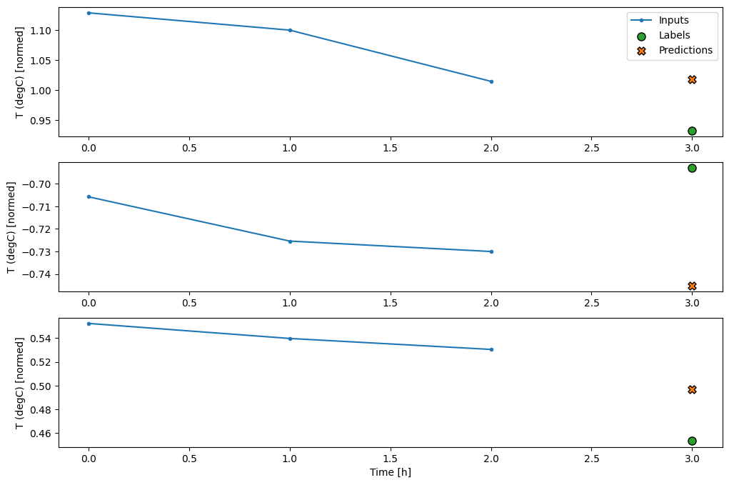
这种方法的主要缺点是,生成的模型只能在具有这种形状的输入窗口上执行。
print('Input shape:', wide_window.example[0].shape)
try:
  print('Output shape:', multi_step_dense(wide_window.example[0]).shape)
except Exception as e:
  print(f'\n{type(e).__name__}:{e}')
Input shape: (32, 24, 19)

ValueError:Exception encountered when calling Sequential.call().

Input 0 of layer "dense_4" is incompatible with the layer: expected axis -1 of input shape to have value 57, but received input with shape (32, 456)

Arguments received by Sequential.call():
  • inputs=tf.Tensor(shape=(32, 24, 19), dtype=float32)
  • training=None
  • mask=None
下一节中的卷积模型解决了这个问题。
卷积神经网络
卷积层 (tf.keras.layers.Conv1D) 也将多个时间步长作为输入到每个预测中。
以下是与 multi_step_dense 相同的模型,使用卷积重新编写。
请注意更改
tf.keras.layers.Flatten和第一个tf.keras.layers.Dense被tf.keras.layers.Conv1D替换。tf.keras.layers.Reshape不再需要,因为卷积在输出中保留时间轴。
conv_model = tf.keras.Sequential([
    tf.keras.layers.Conv1D(filters=32,
                           kernel_size=(CONV_WIDTH,),
                           activation='relu'),
    tf.keras.layers.Dense(units=32, activation='relu'),
    tf.keras.layers.Dense(units=1),
])
在示例批次上运行它,以检查模型是否生成具有预期形状的输出。
print("Conv model on `conv_window`")
print('Input shape:', conv_window.example[0].shape)
print('Output shape:', conv_model(conv_window.example[0]).shape)
Conv model on `conv_window`
Input shape: (32, 3, 19)
Output shape: (32, 1, 1)
在 conv_window 上训练和评估它,它应该提供与 multi_step_dense 模型相似的性能。
history = compile_and_fit(conv_model, conv_window)

IPython.display.clear_output()
val_performance['Conv'] = conv_model.evaluate(conv_window.val, return_dict=True)
performance['Conv'] = conv_model.evaluate(conv_window.test, verbose=0, return_dict=True)
438/438 ━━━━━━━━━━━━━━━━━━━━ 1s 1ms/step - loss: 0.0075 - mean_absolute_error: 0.0615
此 conv_model 与 multi_step_dense 模型之间的区别在于,conv_model 可以运行在任何长度的输入上。卷积层应用于输入的滑动窗口。
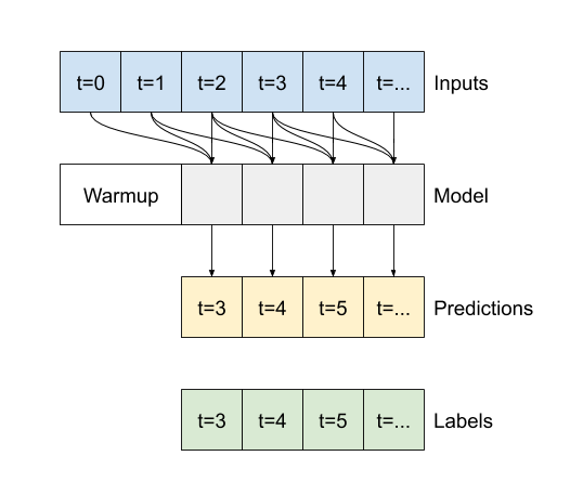
如果您在更宽的输入上运行它,它将生成更宽的输出。
print("Wide window")
print('Input shape:', wide_window.example[0].shape)
print('Labels shape:', wide_window.example[1].shape)
print('Output shape:', conv_model(wide_window.example[0]).shape)
Wide window
Input shape: (32, 24, 19)
Labels shape: (32, 24, 1)
Output shape: (32, 22, 1)
请注意,输出比输入短。为了使训练或绘图工作,您需要标签和预测具有相同的长度。因此,构建一个 WindowGenerator 来生成具有几个额外输入时间步长的宽窗口,以便标签和预测长度匹配。
LABEL_WIDTH = 24
INPUT_WIDTH = LABEL_WIDTH + (CONV_WIDTH - 1)
wide_conv_window = WindowGenerator(
    input_width=INPUT_WIDTH,
    label_width=LABEL_WIDTH,
    shift=1,
    label_columns=['T (degC)'])

wide_conv_window
Total window size: 27
Input indices: [ 0  1  2  3  4  5  6  7  8  9 10 11 12 13 14 15 16 17 18 19 20 21 22 23
 24 25]
Label indices: [ 3  4  5  6  7  8  9 10 11 12 13 14 15 16 17 18 19 20 21 22 23 24 25 26]
Label column name(s): ['T (degC)']
print("Wide conv window")
print('Input shape:', wide_conv_window.example[0].shape)
print('Labels shape:', wide_conv_window.example[1].shape)
print('Output shape:', conv_model(wide_conv_window.example[0]).shape)
Wide conv window
Input shape: (32, 26, 19)
Labels shape: (32, 24, 1)
Output shape: (32, 24, 1)
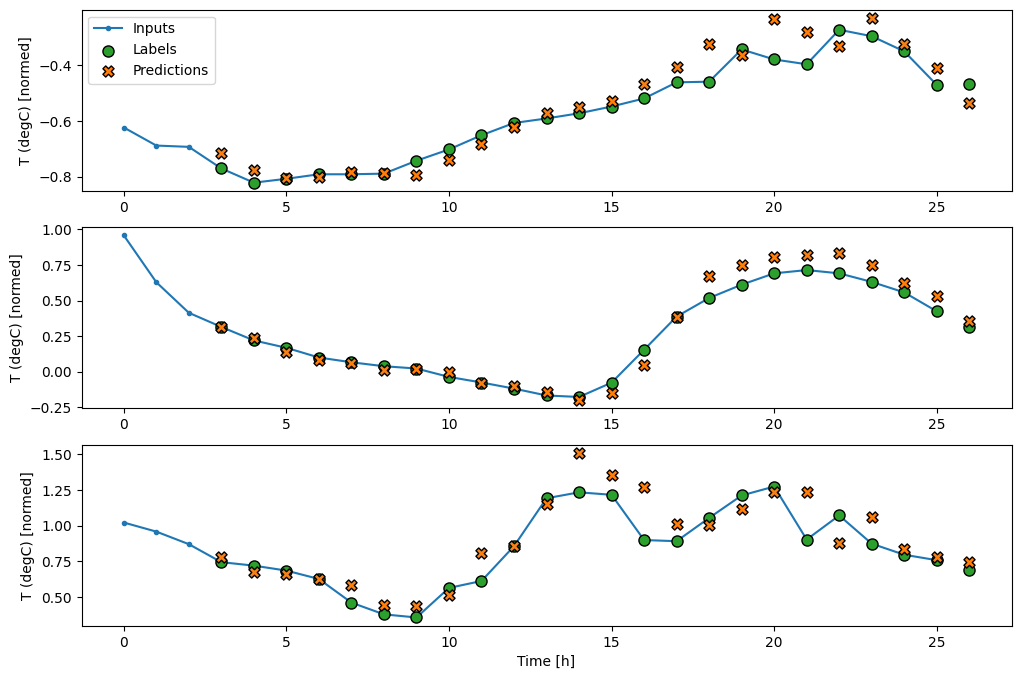
现在,您可以在更宽的窗口上绘制模型的预测。请注意第一个预测之前的 3 个输入时间步长。这里每个预测都基于前 3 个时间步长。
wide_conv_window.plot(conv_model)
循环神经网络
循环神经网络 (RNN) 是一种非常适合时间序列数据的类型的神经网络。RNN 逐个时间步长处理时间序列,并从时间步长到时间步长维护内部状态。
您可以在 使用 RNN 进行文本生成 教程和 使用 Keras 的循环神经网络 (RNN) 指南中了解更多信息。
在本教程中,您将使用一个名为长短期记忆 (tf.keras.layers.LSTM) 的 RNN 层。
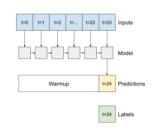
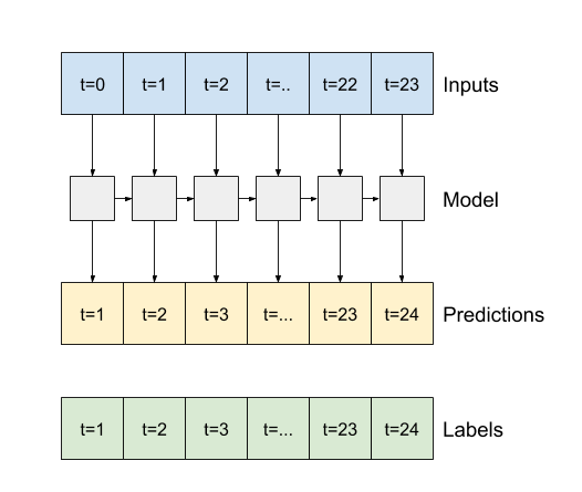
所有 Keras RNN 层(如 tf.keras.layers.LSTM)的重要构造函数参数是 return_sequences 参数。此设置可以以两种方式之一配置层。
- 如果为
False(默认值),则该层仅返回最后一个时间步长的输出,使模型有时间在进行单个预测之前预热其内部状态。
- 如果为
True,则该层将为每个输入返回一个输出。这对于以下情况很有用:- 堆叠 RNN 层。
- 同时在多个时间步长上训练模型。
lstm_model = tf.keras.models.Sequential([
    # Shape [batch, time, features] => [batch, time, lstm_units]
    tf.keras.layers.LSTM(32, return_sequences=True),
    # Shape => [batch, time, features]
    tf.keras.layers.Dense(units=1)
])
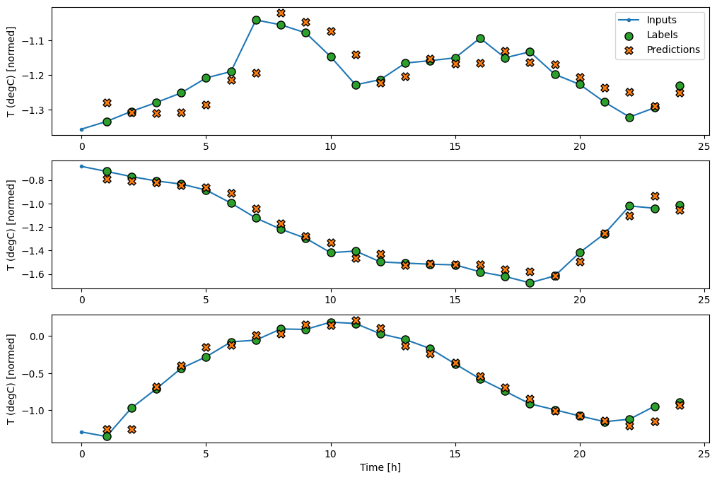
使用 return_sequences=True,模型可以在 24 小时的数据上进行训练。
print('Input shape:', wide_window.example[0].shape)
print('Output shape:', lstm_model(wide_window.example[0]).shape)
Input shape: (32, 24, 19)
Output shape: (32, 24, 1)
history = compile_and_fit(lstm_model, wide_window)

IPython.display.clear_output()
val_performance['LSTM'] = lstm_model.evaluate(wide_window.val, return_dict=True)
performance['LSTM'] = lstm_model.evaluate(wide_window.test, verbose=0, return_dict=True)
438/438 ━━━━━━━━━━━━━━━━━━━━ 1s 2ms/step - loss: 0.0055 - mean_absolute_error: 0.0511
wide_window.plot(lstm_model)
性能
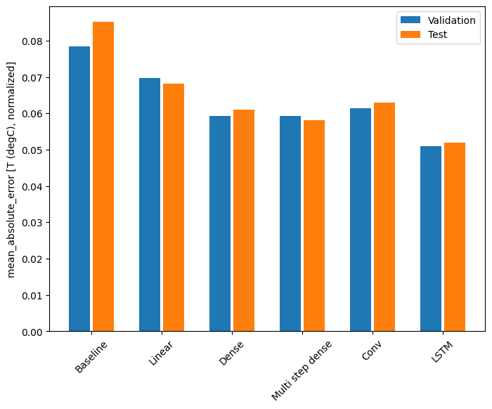
对于此数据集,通常每个模型都比之前的模型略好。
cm = lstm_model.metrics[1]
cm.metrics
[<MeanAbsoluteError name=mean_absolute_error>]
val_performance
{'Baseline': {'loss': 0.012845639139413834,
  'mean_absolute_error': 0.0784662663936615},
 'Linear': {'loss': 0.00884665921330452,
  'mean_absolute_error': 0.0698472261428833},
 'Dense': {'loss': 0.006883115507662296,
  'mean_absolute_error': 0.05929134413599968},
 'Multi step dense': {'loss': 0.006829570047557354,
  'mean_absolute_error': 0.05932893231511116},
 'Conv': {'loss': 0.007479575928300619,
  'mean_absolute_error': 0.06144466996192932},
 'LSTM': {'loss': 0.005511085502803326,
  'mean_absolute_error': 0.050988875329494476} }
x = np.arange(len(performance))
width = 0.3
metric_name = 'mean_absolute_error'
val_mae = [v[metric_name] for v in val_performance.values()]
test_mae = [v[metric_name] for v in performance.values()]

plt.ylabel('mean_absolute_error [T (degC), normalized]')
plt.bar(x - 0.17, val_mae, width, label='Validation')
plt.bar(x + 0.17, test_mae, width, label='Test')
plt.xticks(ticks=x, labels=performance.keys(),
           rotation=45)
_ = plt.legend()
for name, value in performance.items():
  print(f'{name:12s}: {value[metric_name]:0.4f}')
Baseline    : 0.0852
Linear      : 0.0683
Dense       : 0.0611
Multi step dense: 0.0582
Conv        : 0.0629
LSTM        : 0.0520
多输出模型
到目前为止,所有模型都预测了单个输出特征 T (degC),用于单个时间步长。
所有这些模型都可以通过更改输出层中的单元数量并将训练窗口调整为在 labels (example_labels) 中包含所有特征来转换为预测多个特征。
single_step_window = WindowGenerator(
    # `WindowGenerator` returns all features as labels if you
    # don't set the `label_columns` argument.
    input_width=1, label_width=1, shift=1)

wide_window = WindowGenerator(
    input_width=24, label_width=24, shift=1)

for example_inputs, example_labels in wide_window.train.take(1):
  print(f'Inputs shape (batch, time, features): {example_inputs.shape}')
  print(f'Labels shape (batch, time, features): {example_labels.shape}')
Inputs shape (batch, time, features): (32, 24, 19)
Labels shape (batch, time, features): (32, 24, 19)
2024-06-30 02:54:37.053087: W tensorflow/core/framework/local_rendezvous.cc:404] Local rendezvous is aborting with status: OUT_OF_RANGE: End of sequence
请注意,标签的 features 轴现在具有与输入相同的深度,而不是 1。
基线
这里可以使用相同的基线模型 (Baseline),但这次重复所有特征,而不是选择特定的 label_index。
baseline = Baseline()
baseline.compile(loss=tf.keras.losses.MeanSquaredError(),
                 metrics=[tf.keras.metrics.MeanAbsoluteError()])
val_performance = {}
performance = {}
val_performance['Baseline'] = baseline.evaluate(wide_window.val, return_dict=True)
performance['Baseline'] = baseline.evaluate(wide_window.test, verbose=0, return_dict=True)
438/438 ━━━━━━━━━━━━━━━━━━━━ 1s 1ms/step - loss: 0.0885 - mean_absolute_error: 0.1588
Dense
dense = tf.keras.Sequential([
    tf.keras.layers.Dense(units=64, activation='relu'),
    tf.keras.layers.Dense(units=64, activation='relu'),
    tf.keras.layers.Dense(units=num_features)
])
history = compile_and_fit(dense, single_step_window)

IPython.display.clear_output()
val_performance['Dense'] = dense.evaluate(single_step_window.val, return_dict=True)
performance['Dense'] = dense.evaluate(single_step_window.test, verbose=0, return_dict=True)
439/439 ━━━━━━━━━━━━━━━━━━━━ 1s 1ms/step - loss: 0.0665 - mean_absolute_error: 0.1280
RNN
%%time
wide_window = WindowGenerator(
    input_width=24, label_width=24, shift=1)

lstm_model = tf.keras.models.Sequential([
    # Shape [batch, time, features] => [batch, time, lstm_units]
    tf.keras.layers.LSTM(32, return_sequences=True),
    # Shape => [batch, time, features]
    tf.keras.layers.Dense(units=num_features)
])

history = compile_and_fit(lstm_model, wide_window)

IPython.display.clear_output()
val_performance['LSTM'] = lstm_model.evaluate( wide_window.val, return_dict=True)
performance['LSTM'] = lstm_model.evaluate( wide_window.test, verbose=0, return_dict=True)

print()
438/438 ━━━━━━━━━━━━━━━━━━━━ 1s 2ms/step - loss: 0.0614 - mean_absolute_error: 0.1205

CPU times: user 4min 8s, sys: 48.8 s, total: 4min 57s
Wall time: 1min 48s
高级:残差连接
早期的 Baseline 模型利用了序列不会从时间步长到时间步长发生大幅变化的事实。在本教程中训练的每个模型都进行了随机初始化,然后必须学习输出是前一个时间步长的微小变化。
虽然您可以通过仔细的初始化来解决这个问题,但将其构建到模型结构中更简单。
在时间序列分析中,通常构建的模型不是预测下一个值,而是预测下一个时间步长的值将如何变化。类似地,深度学习中的 残差网络(或 ResNets)是指每个层都添加到模型累积结果的架构。
这就是您如何利用变化应该很小的知识。
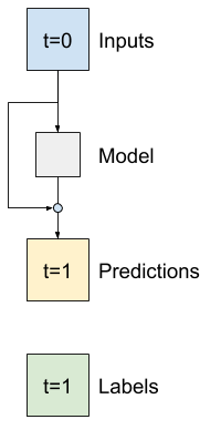
从本质上讲,这将模型初始化为匹配 Baseline。对于此任务,它有助于模型更快地收敛,性能略好。
这种方法可以与本教程中讨论的任何模型结合使用。
在这里,它被应用于 LSTM 模型,请注意使用 tf.initializers.zeros 来确保初始预测的变化很小,并且不会压倒残差连接。这里没有梯度对称性问题,因为 zeros 仅用于最后一层。
class ResidualWrapper(tf.keras.Model):
  def __init__(self, model):
    super().__init__()
    self.model = model

  def call(self, inputs, *args, **kwargs):
    delta = self.model(inputs, *args, **kwargs)

    # The prediction for each time step is the input
    # from the previous time step plus the delta
    # calculated by the model.
    return inputs + delta
%%time
residual_lstm = ResidualWrapper(
    tf.keras.Sequential([
    tf.keras.layers.LSTM(32, return_sequences=True),
    tf.keras.layers.Dense(
        num_features,
        # The predicted deltas should start small.
        # Therefore, initialize the output layer with zeros.
        kernel_initializer=tf.initializers.zeros())
]))

history = compile_and_fit(residual_lstm, wide_window)

IPython.display.clear_output()
val_performance['Residual LSTM'] = residual_lstm.evaluate(wide_window.val, return_dict=True)
performance['Residual LSTM'] = residual_lstm.evaluate(wide_window.test, verbose=0, return_dict=True)
print()
438/438 ━━━━━━━━━━━━━━━━━━━━ 1s 2ms/step - loss: 0.0619 - mean_absolute_error: 0.1179

CPU times: user 1min 51s, sys: 22.2 s, total: 2min 13s
Wall time: 49.4 s
性能
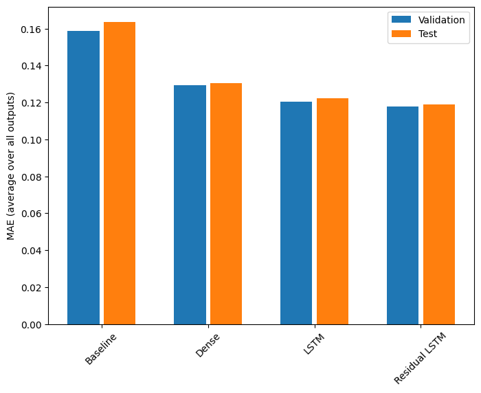
以下是这些多输出模型的整体性能。
x = np.arange(len(performance))
width = 0.3

metric_name = 'mean_absolute_error'
val_mae = [v[metric_name] for v in val_performance.values()]
test_mae = [v[metric_name] for v in performance.values()]

plt.bar(x - 0.17, val_mae, width, label='Validation')
plt.bar(x + 0.17, test_mae, width, label='Test')
plt.xticks(ticks=x, labels=performance.keys(),
           rotation=45)
plt.ylabel('MAE (average over all outputs)')
_ = plt.legend()
for name, value in performance.items():
  print(f'{name:15s}: {value[metric_name]:0.4f}')
Baseline       : 0.1638
Dense          : 0.1307
LSTM           : 0.1223
Residual LSTM  : 0.1191
以上性能是在所有模型输出上平均得到的。
多步模型
上一节中的单输出和多输出模型都进行了单时间步长预测,预测未来一小时。
本节介绍如何扩展这些模型以进行多时间步长预测。
在多步预测中,模型需要学习预测一系列未来值。因此,与仅预测单个未来点的单步模型不同,多步模型预测未来值的序列。
对此有两种大致的方法:
- 一次性预测,其中整个时间序列被一次预测。
- 自回归预测,模型仅进行单步预测,其输出作为其输入反馈。
在本节中,所有模型将预测**所有输出时间步的所有特征**。
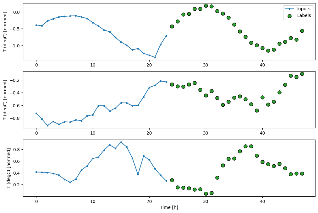
对于多步模型,训练数据仍然由每小时样本组成。但是,在这里,模型将学习在给定过去 24 小时的前提下预测未来 24 小时。
这是一个Window对象,它从数据集中生成这些切片
OUT_STEPS = 24
multi_window = WindowGenerator(input_width=24,
                               label_width=OUT_STEPS,
                               shift=OUT_STEPS)

multi_window.plot()
multi_window
Total window size: 48
Input indices: [ 0  1  2  3  4  5  6  7  8  9 10 11 12 13 14 15 16 17 18 19 20 21 22 23]
Label indices: [24 25 26 27 28 29 30 31 32 33 34 35 36 37 38 39 40 41 42 43 44 45 46 47]
Label column name(s): None
基准
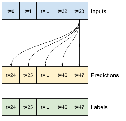
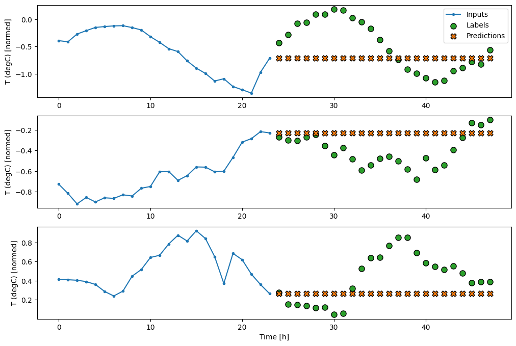
此任务的一个简单基准是将最后一个输入时间步重复所需的输出时间步数。
class MultiStepLastBaseline(tf.keras.Model):
  def call(self, inputs):
    return tf.tile(inputs[:, -1:, :], [1, OUT_STEPS, 1])

last_baseline = MultiStepLastBaseline()
last_baseline.compile(loss=tf.keras.losses.MeanSquaredError(),
                      metrics=[tf.keras.metrics.MeanAbsoluteError()])

multi_val_performance = {}
multi_performance = {}

multi_val_performance['Last'] = last_baseline.evaluate(multi_window.val, return_dict=True)
multi_performance['Last'] = last_baseline.evaluate(multi_window.test, verbose=0, return_dict=True)
multi_window.plot(last_baseline)
437/437 ━━━━━━━━━━━━━━━━━━━━ 1s 2ms/step - loss: 0.6305 - mean_absolute_error: 0.5020
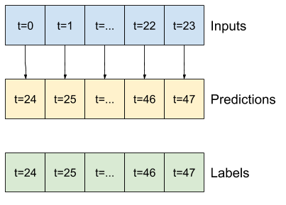
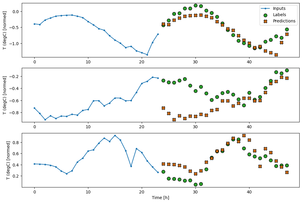
由于此任务是在给定过去 24 小时的前提下预测未来 24 小时,因此另一种简单的方法是重复前一天,假设明天会类似。
class RepeatBaseline(tf.keras.Model):
  def call(self, inputs):
    return inputs

repeat_baseline = RepeatBaseline()
repeat_baseline.compile(loss=tf.keras.losses.MeanSquaredError(),
                        metrics=[tf.keras.metrics.MeanAbsoluteError()])

multi_val_performance['Repeat'] = repeat_baseline.evaluate(multi_window.val, return_dict=True)
multi_performance['Repeat'] = repeat_baseline.evaluate(multi_window.test, verbose=0, return_dict=True)
multi_window.plot(repeat_baseline)
437/437 ━━━━━━━━━━━━━━━━━━━━ 1s 1ms/step - loss: 0.4276 - mean_absolute_error: 0.3954
单次模型
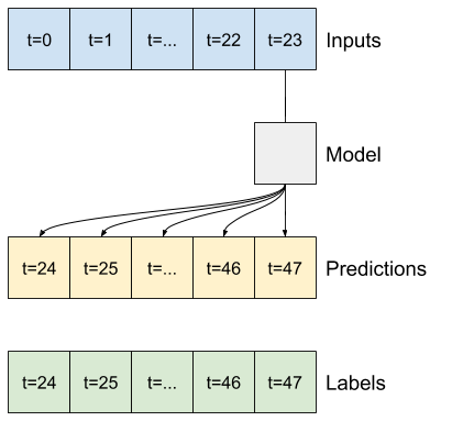
解决此问题的一种高级方法是使用“单次”模型,其中模型在一步内完成整个序列预测。
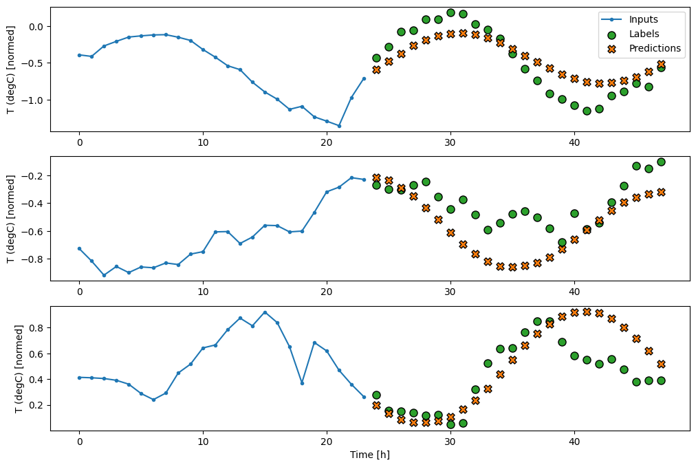
这可以有效地实现为一个tf.keras.layers.Dense,具有OUT_STEPS*features个输出单元。模型只需要将该输出重塑为所需的(OUTPUT_STEPS, features)。
线性
基于最后一个输入时间步的简单线性模型比任何基准都更好,但功能不足。模型需要从单个输入时间步预测OUTPUT_STEPS个时间步,并进行线性投影。它只能捕获行为的低维切片,可能主要基于一天中的时间和一年中的时间。
multi_linear_model = tf.keras.Sequential([
    # Take the last time-step.
    # Shape [batch, time, features] => [batch, 1, features]
    tf.keras.layers.Lambda(lambda x: x[:, -1:, :]),
    # Shape => [batch, 1, out_steps*features]
    tf.keras.layers.Dense(OUT_STEPS*num_features,
                          kernel_initializer=tf.initializers.zeros()),
    # Shape => [batch, out_steps, features]
    tf.keras.layers.Reshape([OUT_STEPS, num_features])
])

history = compile_and_fit(multi_linear_model, multi_window)

IPython.display.clear_output()
multi_val_performance['Linear'] = multi_linear_model.evaluate(multi_window.val, return_dict=True)
multi_performance['Linear'] = multi_linear_model.evaluate(multi_window.test, verbose=0, return_dict=True)
multi_window.plot(multi_linear_model)
437/437 ━━━━━━━━━━━━━━━━━━━━ 1s 1ms/step - loss: 0.2523 - mean_absolute_error: 0.3035
Dense
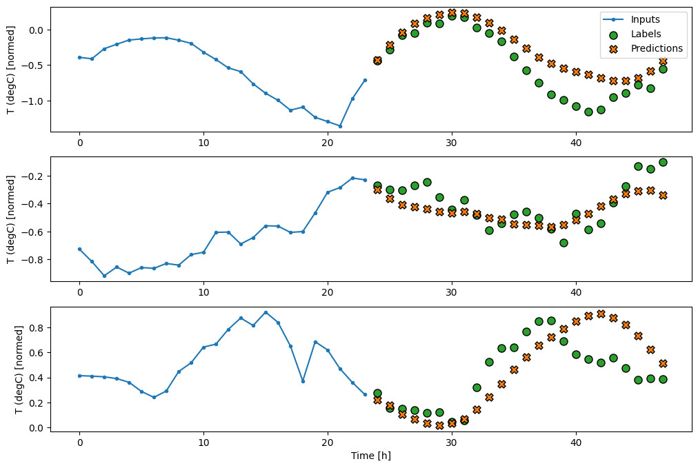
在输入和输出之间添加一个tf.keras.layers.Dense,可以增强线性模型的功能,但它仍然只基于单个输入时间步。
multi_dense_model = tf.keras.Sequential([
    # Take the last time step.
    # Shape [batch, time, features] => [batch, 1, features]
    tf.keras.layers.Lambda(lambda x: x[:, -1:, :]),
    # Shape => [batch, 1, dense_units]
    tf.keras.layers.Dense(512, activation='relu'),
    # Shape => [batch, out_steps*features]
    tf.keras.layers.Dense(OUT_STEPS*num_features,
                          kernel_initializer=tf.initializers.zeros()),
    # Shape => [batch, out_steps, features]
    tf.keras.layers.Reshape([OUT_STEPS, num_features])
])

history = compile_and_fit(multi_dense_model, multi_window)

IPython.display.clear_output()
multi_val_performance['Dense'] = multi_dense_model.evaluate(multi_window.val, return_dict=True)
multi_performance['Dense'] = multi_dense_model.evaluate(multi_window.test, verbose=0, return_dict=True)
multi_window.plot(multi_dense_model)
437/437 ━━━━━━━━━━━━━━━━━━━━ 1s 1ms/step - loss: 0.2158 - mean_absolute_error: 0.2793
CNN
卷积模型根据固定宽度历史进行预测,这可能比密集模型具有更好的性能,因为它可以查看事物如何随时间变化。
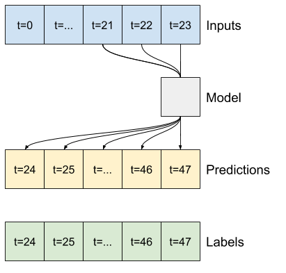
CONV_WIDTH = 3
multi_conv_model = tf.keras.Sequential([
    # Shape [batch, time, features] => [batch, CONV_WIDTH, features]
    tf.keras.layers.Lambda(lambda x: x[:, -CONV_WIDTH:, :]),
    # Shape => [batch, 1, conv_units]
    tf.keras.layers.Conv1D(256, activation='relu', kernel_size=(CONV_WIDTH)),
    # Shape => [batch, 1,  out_steps*features]
    tf.keras.layers.Dense(OUT_STEPS*num_features,
                          kernel_initializer=tf.initializers.zeros()),
    # Shape => [batch, out_steps, features]
    tf.keras.layers.Reshape([OUT_STEPS, num_features])
])

history = compile_and_fit(multi_conv_model, multi_window)

IPython.display.clear_output()

multi_val_performance['Conv'] = multi_conv_model.evaluate(multi_window.val, return_dict=True)
multi_performance['Conv'] = multi_conv_model.evaluate(multi_window.test, verbose=0, return_dict=True)
multi_window.plot(multi_conv_model)
437/437 ━━━━━━━━━━━━━━━━━━━━ 1s 1ms/step - loss: 0.2154 - mean_absolute_error: 0.2798
RNN
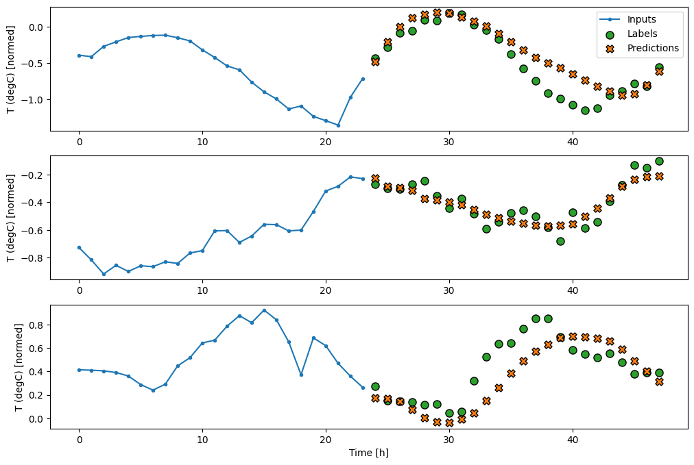
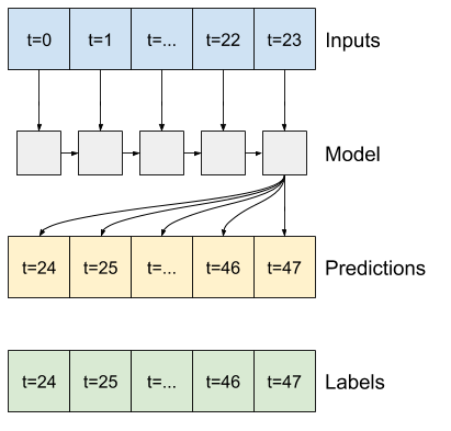
循环模型可以学习使用长时间的输入历史,如果它与模型正在进行的预测相关。在这里,模型将在进行未来 24 小时的单个预测之前积累 24 小时的内部状态。
在这种单次格式中,LSTM 只需要在最后一个时间步产生输出,因此在tf.keras.layers.LSTM中设置return_sequences=False。
multi_lstm_model = tf.keras.Sequential([
    # Shape [batch, time, features] => [batch, lstm_units].
    # Adding more `lstm_units` just overfits more quickly.
    tf.keras.layers.LSTM(32, return_sequences=False),
    # Shape => [batch, out_steps*features].
    tf.keras.layers.Dense(OUT_STEPS*num_features,
                          kernel_initializer=tf.initializers.zeros()),
    # Shape => [batch, out_steps, features].
    tf.keras.layers.Reshape([OUT_STEPS, num_features])
])

history = compile_and_fit(multi_lstm_model, multi_window)

IPython.display.clear_output()

multi_val_performance['LSTM'] = multi_lstm_model.evaluate(multi_window.val, return_dict=True)
multi_performance['LSTM'] = multi_lstm_model.evaluate(multi_window.test, verbose=0, return_dict=True)
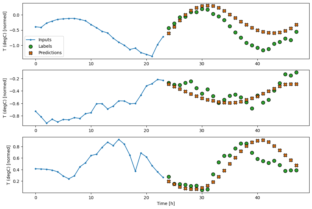
multi_window.plot(multi_lstm_model)
437/437 ━━━━━━━━━━━━━━━━━━━━ 1s 2ms/step - loss: 0.2132 - mean_absolute_error: 0.2829
高级:自回归模型
以上所有模型都在一步内预测整个输出序列。
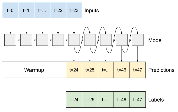
在某些情况下,模型将此预测分解为各个时间步可能会有所帮助。然后,每个模型的输出可以在每个步骤中反馈到自身,并且可以根据前一个预测进行预测,就像经典的使用循环神经网络生成序列一样。
这种模型风格的一个明显优势是它可以设置为生成长度可变的输出。
您可以使用本教程前半部分训练的任何单步多输出模型,并在自回归反馈循环中运行,但在这里您将专注于构建一个明确训练为执行此操作的模型。
RNN
本教程只构建了一个自回归 RNN 模型,但这种模式可以应用于任何旨在输出单个时间步的模型。
该模型将具有与早期单步 LSTM 模型相同的基本形式:一个tf.keras.layers.LSTM层,后面跟着一个tf.keras.layers.Dense层,将LSTM层的输出转换为模型预测。
一个tf.keras.layers.LSTM是一个tf.keras.layers.LSTMCell,它包装在更高级别的tf.keras.layers.RNN中,该层为您管理状态和序列结果(查看使用 Keras 的循环神经网络 (RNN)指南了解详细信息)。
在这种情况下,模型必须手动管理每个步骤的输入,因此它直接使用tf.keras.layers.LSTMCell来实现更低级别的单时间步接口。
class FeedBack(tf.keras.Model):
  def __init__(self, units, out_steps):
    super().__init__()
    self.out_steps = out_steps
    self.units = units
    self.lstm_cell = tf.keras.layers.LSTMCell(units)
    # Also wrap the LSTMCell in an RNN to simplify the `warmup` method.
    self.lstm_rnn = tf.keras.layers.RNN(self.lstm_cell, return_state=True)
    self.dense = tf.keras.layers.Dense(num_features)
feedback_model = FeedBack(units=32, out_steps=OUT_STEPS)
此模型需要的第一个方法是warmup方法,用于根据输入初始化其内部状态。训练后,此状态将捕获输入历史的相关部分。这等效于早期的单步LSTM模型。
def warmup(self, inputs):
  # inputs.shape => (batch, time, features)
  # x.shape => (batch, lstm_units)
  x, *state = self.lstm_rnn(inputs)

  # predictions.shape => (batch, features)
  prediction = self.dense(x)
  return prediction, state

FeedBack.warmup = warmup
此方法返回单个时间步预测和LSTM的内部状态。
prediction, state = feedback_model.warmup(multi_window.example[0])
prediction.shape
TensorShape([32, 19])
有了RNN的状态和初始预测,您现在可以继续迭代模型,将每个步骤的预测作为输入反馈。
收集输出预测的最简单方法是使用 Python 列表和循环后的tf.stack。
def call(self, inputs, training=None):
  # Use a TensorArray to capture dynamically unrolled outputs.
  predictions = []
  # Initialize the LSTM state.
  prediction, state = self.warmup(inputs)

  # Insert the first prediction.
  predictions.append(prediction)

  # Run the rest of the prediction steps.
  for n in range(1, self.out_steps):
    # Use the last prediction as input.
    x = prediction
    # Execute one lstm step.
    x, state = self.lstm_cell(x, states=state,
                              training=training)
    # Convert the lstm output to a prediction.
    prediction = self.dense(x)
    # Add the prediction to the output.
    predictions.append(prediction)

  # predictions.shape => (time, batch, features)
  predictions = tf.stack(predictions)
  # predictions.shape => (batch, time, features)
  predictions = tf.transpose(predictions, [1, 0, 2])
  return predictions

FeedBack.call = call
在示例输入上运行此模型。
print('Output shape (batch, time, features): ', feedback_model(multi_window.example[0]).shape)
Output shape (batch, time, features): (32, 24, 19)
现在,训练模型。
history = compile_and_fit(feedback_model, multi_window)

IPython.display.clear_output()

multi_val_performance['AR LSTM'] = feedback_model.evaluate(multi_window.val, return_dict=True)
multi_performance['AR LSTM'] = feedback_model.evaluate(multi_window.test, verbose=0, return_dict=True)
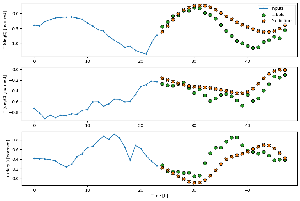
multi_window.plot(feedback_model)
437/437 ━━━━━━━━━━━━━━━━━━━━ 1s 2ms/step - loss: 0.2277 - mean_absolute_error: 0.3026
性能
作为模型复杂性的函数,显然存在边际收益递减。
x = np.arange(len(multi_performance))
width = 0.3

metric_name = 'mean_absolute_error'
val_mae = [v[metric_name] for v in multi_val_performance.values()]
test_mae = [v[metric_name] for v in multi_performance.values()]

plt.bar(x - 0.17, val_mae, width, label='Validation')
plt.bar(x + 0.17, test_mae, width, label='Test')
plt.xticks(ticks=x, labels=multi_performance.keys(),
           rotation=45)
plt.ylabel(f'MAE (average over all times and outputs)')
_ = plt.legend()
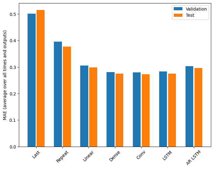
本教程前半部分中多输出模型的指标显示了所有输出特征的平均性能。这些性能相似,但也跨输出时间步平均。
for name, value in multi_performance.items():
  print(f'{name:8s}: {value[metric_name]:0.4f}')
Last    : 0.5157
Repeat  : 0.3774
Linear  : 0.2984
Dense   : 0.2754
Conv    : 0.2723
LSTM    : 0.2745
AR LSTM : 0.2958
从密集模型到卷积模型和循环模型的改进只有百分之几(如果有的话),而自回归模型的性能明显更差。因此,这些更复杂的方法可能不值得在**此**问题上使用,但没有尝试就无法知道,这些模型可能对**您的**问题有所帮助。
下一步
本教程是使用 TensorFlow 进行时间序列预测的快速入门。
要了解更多信息,请参阅
- 动手学机器学习:Scikit-Learn、Keras 和 TensorFlow第 15 章,第二版。
- Python 深度学习第 6 章。
- Udacity 的深度学习 TensorFlow 入门第 8 课,包括练习笔记本。
另外,请记住,您可以在 TensorFlow 中实现任何经典时间序列模型——本教程只关注 TensorFlow 的内置功能。