带注意力机制的神经机器翻译

本教程演示了如何训练一个用于西班牙语到英语翻译的序列到序列（seq2seq）模型，该模型大致基于《Effective Approaches to Attention-based Neural Machine Translation》（Luong 等人，2015 年）。

本教程内容：一个通过注意力机制连接的编码器/解码器。

虽然这种架构已经有些过时，但它仍然是一个非常有用的练习项目，可以让你在深入学习序列到序列模型和注意力机制（在此之后可以学习Transformer）之前，获得更深刻的理解。

本示例假设您具备一些低于 Keras 层级别的 TensorFlow 基础知识

在本笔记本中完成模型训练后，您将能够输入一个西班牙语句子，例如“¿todavia estan en casa?”，并得到相应的英语翻译：“are you still at home?”

生成的模型可以导出为 tf.saved_model，因此可以在其他 TensorFlow 环境中使用。

对于一个演示示例来说，翻译质量是合理的，但生成的注意力图可能更有趣。它显示了模型在翻译过程中注意力集中在输入句子的哪些部分。

spanish-english attention plot

设置

pip install "tensorflow-text>=2.11"
pip install einops

import numpy as np

import typing
from typing import Any, Tuple

import einops
import matplotlib.pyplot as plt
import matplotlib.ticker as ticker

import tensorflow as tf
import tensorflow_text as tf_text

本教程使用了很多底层 API，很容易搞错形状（shapes）。此类用于在整个教程中检查形状。

class ShapeChecker():
  def __init__(self):
    # Keep a cache of every axis-name seen
    self.shapes = {}

  def __call__(self, tensor, names, broadcast=False):
    if not tf.executing_eagerly():
      return

    parsed = einops.parse_shape(tensor, names)

    for name, new_dim in parsed.items():
      old_dim = self.shapes.get(name, None)

      if (broadcast and new_dim == 1):
        continue

      if old_dim is None:
        # If the axis name is new, add its length to the cache.
        self.shapes[name] = new_dim
        continue

      if new_dim != old_dim:
        raise ValueError(f"Shape mismatch for dimension: '{name}'\n"
                         f"    found: {new_dim}\n"
                         f"    expected: {old_dim}\n")

数据

本教程使用了由 Anki 提供的语言数据集。该数据集包含以下格式的语言翻译对：

May I borrow this book? ¿Puedo tomar prestado este libro?

他们提供了多种语言，但本示例使用的是英西数据集。

下载并准备数据集

为了方便起见，该数据集的一个副本托管在 Google Cloud 上，但您也可以下载自己的副本。下载数据集后，您需要采取以下步骤来准备数据：

为每个句子添加开始和结束标记。
通过删除特殊字符来清理句子。
创建词索引和反向词索引（映射单词 → ID 和 ID → 单词的字典）。
将每个句子填充（Pad）到最大长度。

# Download the file
import pathlib

path_to_zip = tf.keras.utils.get_file(
    'spa-eng.zip', origin='http://storage.googleapis.com/download.tensorflow.org/data/spa-eng.zip',
    extract=True)

path_to_file = pathlib.Path(path_to_zip).parent/'spa-eng/spa.txt'

def load_data(path):
  text = path.read_text(encoding='utf-8')

  lines = text.splitlines()
  pairs = [line.split('\t') for line in lines]

  context = np.array([context for target, context in pairs])
  target = np.array([target for target, context in pairs])

  return target, context

target_raw, context_raw = load_data(path_to_file)
print(context_raw[-1])

print(target_raw[-1])

创建 tf.data 数据集

您可以从这些字符串数组中创建一个字符串 tf.data.Dataset，以高效地对其进行打乱和分批处理。

BUFFER_SIZE = len(context_raw)
BATCH_SIZE = 64

is_train = np.random.uniform(size=(len(target_raw),)) < 0.8

train_raw = (
    tf.data.Dataset
    .from_tensor_slices((context_raw[is_train], target_raw[is_train]))
    .shuffle(BUFFER_SIZE)
    .batch(BATCH_SIZE))
val_raw = (
    tf.data.Dataset
    .from_tensor_slices((context_raw[~is_train], target_raw[~is_train]))
    .shuffle(BUFFER_SIZE)
    .batch(BATCH_SIZE))

for example_context_strings, example_target_strings in train_raw.take(1):
  print(example_context_strings[:5])
  print()
  print(example_target_strings[:5])
  break

文本预处理

本教程的目标之一是构建一个可以导出为 tf.saved_model 的模型。为了使导出的模型有用，它应该接收 tf.string 输入，并返回 tf.string 输出：所有的文本处理都在模型内部进行，主要使用 layers.TextVectorization 层。

标准化

该模型处理的是词汇量有限的多语言文本。因此，标准化输入文本非常重要。

第一步是进行 Unicode 标准化，以拆分重音字符并将兼容字符替换为其 ASCII 等效字符。

tensorflow_text 包中包含一个 unicode 标准化操作。

example_text = tf.constant('¿Todavía está en casa?')

print(example_text.numpy())
print(tf_text.normalize_utf8(example_text, 'NFKD').numpy())

Unicode 标准化将是文本标准化函数中的第一步。

def tf_lower_and_split_punct(text):
  # Split accented characters.
  text = tf_text.normalize_utf8(text, 'NFKD')
  text = tf.strings.lower(text)
  # Keep space, a to z, and select punctuation.
  text = tf.strings.regex_replace(text, '[^ a-z.?!,¿]', '')
  # Add spaces around punctuation.
  text = tf.strings.regex_replace(text, '[.?!,¿]', r' \0 ')
  # Strip whitespace.
  text = tf.strings.strip(text)

  text = tf.strings.join(['[START]', text, '[END]'], separator=' ')
  return text

print(example_text.numpy().decode())
print(tf_lower_and_split_punct(example_text).numpy().decode())

文本向量化

此标准化函数将被封装在 tf.keras.layers.TextVectorization 层中，该层将处理词汇表提取以及将输入文本转换为标记（token）序列。

max_vocab_size = 5000

context_text_processor = tf.keras.layers.TextVectorization(
    standardize=tf_lower_and_split_punct,
    max_tokens=max_vocab_size,
    ragged=True)

TextVectorization 层和许多其他 Keras 预处理层都有一个 adapt 方法。此方法读取一个 epoch 的训练数据，其工作方式与 Model.fit 非常相似。该 adapt 方法会根据数据初始化该层。在这里，它确定了词汇表。

context_text_processor.adapt(train_raw.map(lambda context, target: context))

# Here are the first 10 words from the vocabulary:
context_text_processor.get_vocabulary()[:10]

这就是西班牙语的 TextVectorization 层，现在构建并 .adapt() 英语层。

target_text_processor = tf.keras.layers.TextVectorization(
    standardize=tf_lower_and_split_punct,
    max_tokens=max_vocab_size,
    ragged=True)

target_text_processor.adapt(train_raw.map(lambda context, target: target))
target_text_processor.get_vocabulary()[:10]

现在这些层可以将一批字符串转换为一批标记 ID。

example_tokens = context_text_processor(example_context_strings)
example_tokens[:3, :]

get_vocabulary 方法可用于将标记 ID 转回文本。

context_vocab = np.array(context_text_processor.get_vocabulary())
tokens = context_vocab[example_tokens[0].numpy()]
' '.join(tokens)

返回的标记 ID 是零填充（zero-padded）的。这可以很容易地转换为掩码（mask）。

plt.subplot(1, 2, 1)
plt.pcolormesh(example_tokens.to_tensor())
plt.title('Token IDs')

plt.subplot(1, 2, 2)
plt.pcolormesh(example_tokens.to_tensor() != 0)
plt.title('Mask')

处理数据集

下面的 process_text 函数将字符串 Dataset 转换为 0 填充的标记 ID 张量。它还通过 keras.Model.fit 将 (context, target) 对转换为用于训练的 ((context, target_in), target_out) 对。Keras 期望 (inputs, labels) 对，输入是 (context, target_in)，标签是 target_out。target_in 和 target_out 之间的区别在于它们相对于彼此偏移了一个位置，因此在每个位置，标签都是下一个标记。

def process_text(context, target):
  context = context_text_processor(context).to_tensor()
  target = target_text_processor(target)
  targ_in = target[:,:-1].to_tensor()
  targ_out = target[:,1:].to_tensor()
  return (context, targ_in), targ_out


train_ds = train_raw.map(process_text, tf.data.AUTOTUNE)
val_ds = val_raw.map(process_text, tf.data.AUTOTUNE)

这是来自第一批数据的第一个序列。

for (ex_context_tok, ex_tar_in), ex_tar_out in train_ds.take(1):
  print(ex_context_tok[0, :10].numpy()) 
  print()
  print(ex_tar_in[0, :10].numpy()) 
  print(ex_tar_out[0, :10].numpy())

编码器/解码器

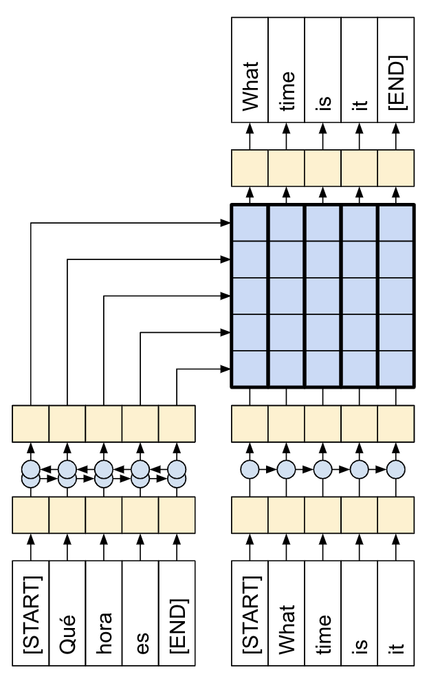
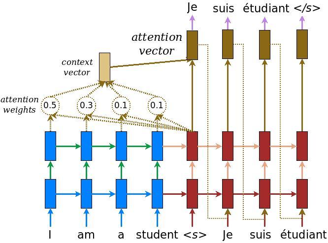
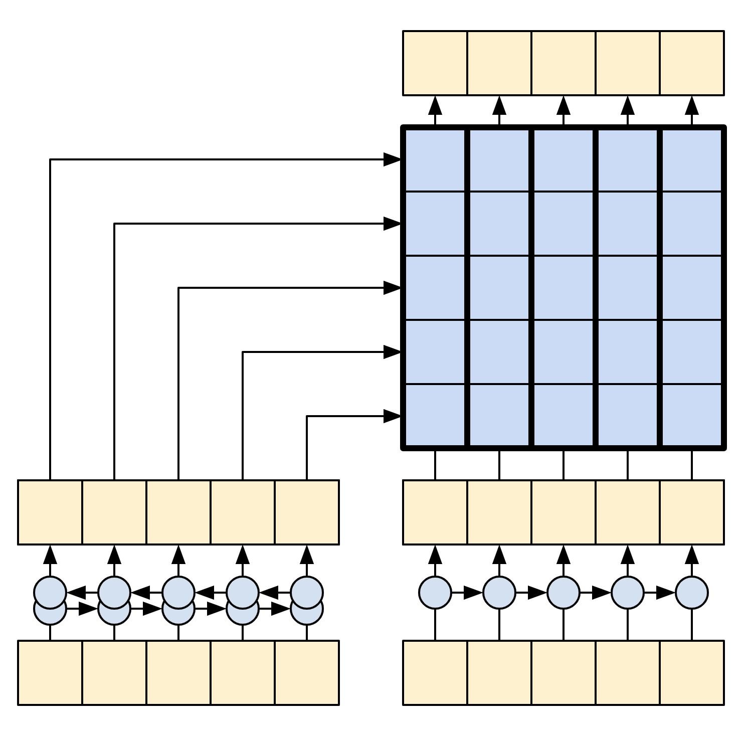
下图展示了模型的概览。在这两幅图中，编码器都在左侧，解码器都在右侧。在每个时间步，解码器的输出都会与编码器的输出相结合，以预测下一个单词。

原图 [左] 包含一些额外的连接，在本教程的模型 [右] 中特意省略了，因为它们通常是不必要的，且难以实现。那些缺失的连接是：

将编码器 RNN 的状态馈送到解码器 RNN。
将注意力输出反馈到 RNN 的输入。

摘自《Effective Approaches to Attention-based Neural Machine Translation》的原图。	本教程的模型

在开始之前，先为模型定义常量。

UNITS = 256

编码器

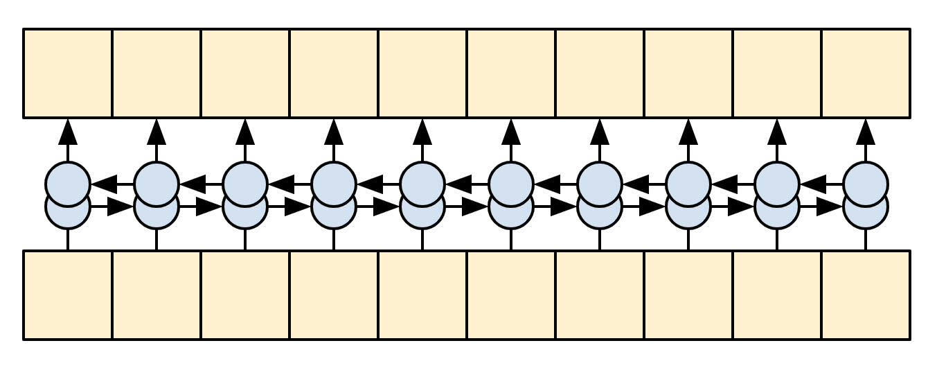
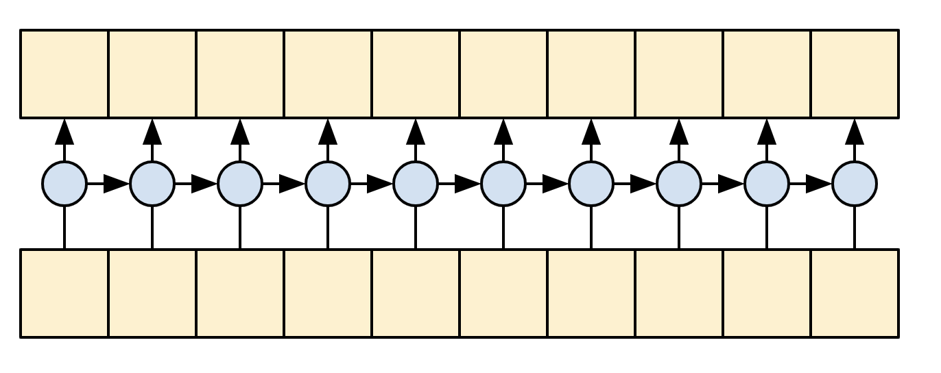
编码器的目标是将上下文序列处理为一系列向量，这些向量对于解码器在尝试预测每个时间步的下一个输出时很有用。由于上下文序列是固定的，因此对编码器中的信息流动方式没有限制，所以我们使用双向 RNN 进行处理。

双向 RNN

编码器

接收一个标记 ID 列表（来自 context_text_processor）。
查找每个标记的嵌入向量（使用 layers.Embedding）。
将嵌入处理为新序列（使用双向 layers.GRU）。
返回处理后的序列。这将传递给注意力头（attention head）。

class Encoder(tf.keras.layers.Layer):
  def __init__(self, text_processor, units):
    super(Encoder, self).__init__()
    self.text_processor = text_processor
    self.vocab_size = text_processor.vocabulary_size()
    self.units = units

    # The embedding layer converts tokens to vectors
    self.embedding = tf.keras.layers.Embedding(self.vocab_size, units,
                                               mask_zero=True)

    # The RNN layer processes those vectors sequentially.
    self.rnn = tf.keras.layers.Bidirectional(
        merge_mode='sum',
        layer=tf.keras.layers.GRU(units,
                            # Return the sequence and state
                            return_sequences=True,
                            recurrent_initializer='glorot_uniform'))

  def call(self, x):
    shape_checker = ShapeChecker()
    shape_checker(x, 'batch s')

    # 2. The embedding layer looks up the embedding vector for each token.
    x = self.embedding(x)
    shape_checker(x, 'batch s units')

    # 3. The GRU processes the sequence of embeddings.
    x = self.rnn(x)
    shape_checker(x, 'batch s units')

    # 4. Returns the new sequence of embeddings.
    return x

  def convert_input(self, texts):
    texts = tf.convert_to_tensor(texts)
    if len(texts.shape) == 0:
      texts = tf.convert_to_tensor(texts)[tf.newaxis]
    context = self.text_processor(texts).to_tensor()
    context = self(context)
    return context

试一试

# Encode the input sequence.
encoder = Encoder(context_text_processor, UNITS)
ex_context = encoder(ex_context_tok)

print(f'Context tokens, shape (batch, s): {ex_context_tok.shape}')
print(f'Encoder output, shape (batch, s, units): {ex_context.shape}')

注意力层

注意力层允许解码器访问由编码器提取的信息。它从整个上下文序列中计算出一个向量，并将其添加到解码器的输出中。

从整个序列计算单个向量的最简单方法是取跨序列的平均值（layers.GlobalAveragePooling1D）。注意力层与之类似，但计算的是上下文序列上的加权平均值。权重由上下文向量和“查询”向量的组合计算得出。

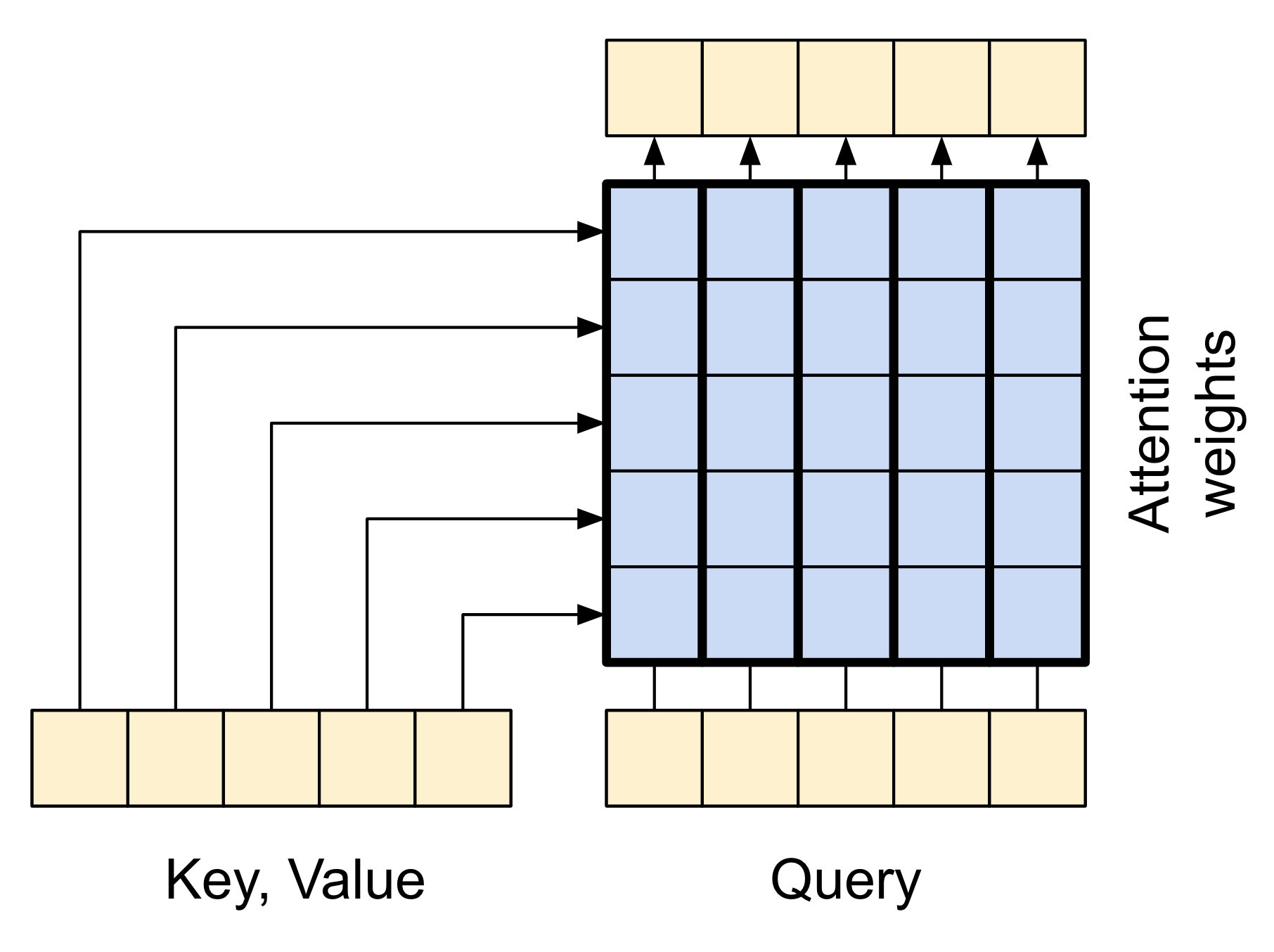
注意力层

class CrossAttention(tf.keras.layers.Layer):
  def __init__(self, units, **kwargs):
    super().__init__()
    self.mha = tf.keras.layers.MultiHeadAttention(key_dim=units, num_heads=1, **kwargs)
    self.layernorm = tf.keras.layers.LayerNormalization()
    self.add = tf.keras.layers.Add()

  def call(self, x, context):
    shape_checker = ShapeChecker()

    shape_checker(x, 'batch t units')
    shape_checker(context, 'batch s units')

    attn_output, attn_scores = self.mha(
        query=x,
        value=context,
        return_attention_scores=True)

    shape_checker(x, 'batch t units')
    shape_checker(attn_scores, 'batch heads t s')

    # Cache the attention scores for plotting later.
    attn_scores = tf.reduce_mean(attn_scores, axis=1)
    shape_checker(attn_scores, 'batch t s')
    self.last_attention_weights = attn_scores

    x = self.add([x, attn_output])
    x = self.layernorm(x)

    return x

attention_layer = CrossAttention(UNITS)

# Attend to the encoded tokens
embed = tf.keras.layers.Embedding(target_text_processor.vocabulary_size(),
                                  output_dim=UNITS, mask_zero=True)
ex_tar_embed = embed(ex_tar_in)

result = attention_layer(ex_tar_embed, ex_context)

print(f'Context sequence, shape (batch, s, units): {ex_context.shape}')
print(f'Target sequence, shape (batch, t, units): {ex_tar_embed.shape}')
print(f'Attention result, shape (batch, t, units): {result.shape}')
print(f'Attention weights, shape (batch, t, s):    {attention_layer.last_attention_weights.shape}')

在目标序列的每个位置，注意力权重在上下文序列上的总和为 1。

attention_layer.last_attention_weights[0].numpy().sum(axis=-1)

这是在 t=0 时上下文序列上的注意力权重。

attention_weights = attention_layer.last_attention_weights
mask=(ex_context_tok != 0).numpy()

plt.subplot(1, 2, 1)
plt.pcolormesh(mask*attention_weights[:, 0, :])
plt.title('Attention weights')

plt.subplot(1, 2, 2)
plt.pcolormesh(mask)
plt.title('Mask');

由于采用了较小值的随机初始化，注意力权重最初都接近 1/(序列长度)。随着训练的进行，模型将学会使这些权重不再那么均匀。

解码器

解码器的任务是为目标序列中每个位置的下一个标记生成预测。

它查找目标序列中每个标记的嵌入。
它使用 RNN 处理目标序列，并跟踪到目前为止已生成的内容。
当关注编码器的输出时，它使用 RNN 输出作为注意力层的“查询”。
它在输出的每个位置预测下一个标记。

训练时，模型在每个位置预测下一个单词。因此，信息在模型中只能沿一个方向流动非常重要。解码器使用单向（非双向）RNN 来处理目标序列。

当使用此模型进行推理时，它一次产生一个单词，并将其反馈回模型中。

单向 RNN

这是 Decoder 类的初始化器。初始化器创建了所有必要的层。

class Decoder(tf.keras.layers.Layer):
  @classmethod
  def add_method(cls, fun):
    setattr(cls, fun.__name__, fun)
    return fun

  def __init__(self, text_processor, units):
    super(Decoder, self).__init__()
    self.text_processor = text_processor
    self.vocab_size = text_processor.vocabulary_size()
    self.word_to_id = tf.keras.layers.StringLookup(
        vocabulary=text_processor.get_vocabulary(),
        mask_token='', oov_token='[UNK]')
    self.id_to_word = tf.keras.layers.StringLookup(
        vocabulary=text_processor.get_vocabulary(),
        mask_token='', oov_token='[UNK]',
        invert=True)
    self.start_token = self.word_to_id('[START]')
    self.end_token = self.word_to_id('[END]')

    self.units = units


    # 1. The embedding layer converts token IDs to vectors
    self.embedding = tf.keras.layers.Embedding(self.vocab_size,
                                               units, mask_zero=True)

    # 2. The RNN keeps track of what's been generated so far.
    self.rnn = tf.keras.layers.GRU(units,
                                   return_sequences=True,
                                   return_state=True,
                                   recurrent_initializer='glorot_uniform')

    # 3. The RNN output will be the query for the attention layer.
    self.attention = CrossAttention(units)

    # 4. This fully connected layer produces the logits for each
    # output token.
    self.output_layer = tf.keras.layers.Dense(self.vocab_size)

训练

接下来是 call 方法，它接收 3 个参数：

inputs - 一个 context, x 对，其中：
- context - 是来自编码器输出的上下文。
- x - 是目标序列输入。
state - 可选，解码器的先前 state 输出（解码器 RNN 的内部状态）。传递先前运行的状态以从中断处继续生成文本。
return_state - [默认: False] - 设置为 True 以返回 RNN 状态。

@Decoder.add_method
def call(self,
         context, x,
         state=None,
         return_state=False):  
  shape_checker = ShapeChecker()
  shape_checker(x, 'batch t')
  shape_checker(context, 'batch s units')

  # 1. Lookup the embeddings
  x = self.embedding(x)
  shape_checker(x, 'batch t units')

  # 2. Process the target sequence.
  x, state = self.rnn(x, initial_state=state)
  shape_checker(x, 'batch t units')

  # 3. Use the RNN output as the query for the attention over the context.
  x = self.attention(x, context)
  self.last_attention_weights = self.attention.last_attention_weights
  shape_checker(x, 'batch t units')
  shape_checker(self.last_attention_weights, 'batch t s')

  # Step 4. Generate logit predictions for the next token.
  logits = self.output_layer(x)
  shape_checker(logits, 'batch t target_vocab_size')

  if return_state:
    return logits, state
  else:
    return logits

这对于训练来说已经足够了。创建一个解码器实例进行测试。

decoder = Decoder(target_text_processor, UNITS)

在训练中，您将这样使用解码器：

给定上下文和目标标记，它为每个目标标记预测下一个目标标记。

logits = decoder(ex_context, ex_tar_in)

print(f'encoder output shape: (batch, s, units) {ex_context.shape}')
print(f'input target tokens shape: (batch, t) {ex_tar_in.shape}')
print(f'logits shape shape: (batch, target_vocabulary_size) {logits.shape}')

推理

要将其用于推理，您还需要几个方法。

@Decoder.add_method
def get_initial_state(self, context):
  batch_size = tf.shape(context)[0]
  start_tokens = tf.fill([batch_size, 1], self.start_token)
  done = tf.zeros([batch_size, 1], dtype=tf.bool)
  embedded = self.embedding(start_tokens)
  return start_tokens, done, self.rnn.get_initial_state(embedded)[0]

@Decoder.add_method
def tokens_to_text(self, tokens):
  words = self.id_to_word(tokens)
  result = tf.strings.reduce_join(words, axis=-1, separator=' ')
  result = tf.strings.regex_replace(result, '^ *\[START\] *', '')
  result = tf.strings.regex_replace(result, ' *\[END\] *$', '')
  return result

@Decoder.add_method
def get_next_token(self, context, next_token, done, state, temperature = 0.0):
  logits, state = self(
    context, next_token,
    state = state,
    return_state=True) 

  if temperature == 0.0:
    next_token = tf.argmax(logits, axis=-1)
  else:
    logits = logits[:, -1, :]/temperature
    next_token = tf.random.categorical(logits, num_samples=1)

  # If a sequence produces an `end_token`, set it `done`
  done = done | (next_token == self.end_token)
  # Once a sequence is done it only produces 0-padding.
  next_token = tf.where(done, tf.constant(0, dtype=tf.int64), next_token)

  return next_token, done, state

有了这些额外的函数，您可以编写一个生成循环。

# Setup the loop variables.
next_token, done, state = decoder.get_initial_state(ex_context)
tokens = []

for n in range(10):
  # Run one step.
  next_token, done, state = decoder.get_next_token(
      ex_context, next_token, done, state, temperature=1.0)
  # Add the token to the output.
  tokens.append(next_token)

# Stack all the tokens together.
tokens = tf.concat(tokens, axis=-1) # (batch, t)

# Convert the tokens back to a a string
result = decoder.tokens_to_text(tokens)
result[:3].numpy()

由于模型未经训练，它几乎是随机且均匀地从词汇表中输出项目。

模型

现在您已经拥有了所有模型组件，将它们组合起来构建用于训练的模型。

class Translator(tf.keras.Model):
  @classmethod
  def add_method(cls, fun):
    setattr(cls, fun.__name__, fun)
    return fun

  def __init__(self, units,
               context_text_processor,
               target_text_processor):
    super().__init__()
    # Build the encoder and decoder
    encoder = Encoder(context_text_processor, units)
    decoder = Decoder(target_text_processor, units)

    self.encoder = encoder
    self.decoder = decoder

  def call(self, inputs):
    context, x = inputs
    context = self.encoder(context)
    logits = self.decoder(context, x)

    #TODO(b/250038731): remove this
    try:
      # Delete the keras mask, so keras doesn't scale the loss+accuracy. 
      del logits._keras_mask
    except AttributeError:
      pass

    return logits

训练期间，模型的使用方式如下：

model = Translator(UNITS, context_text_processor, target_text_processor)

logits = model((ex_context_tok, ex_tar_in))

print(f'Context tokens, shape: (batch, s, units) {ex_context_tok.shape}')
print(f'Target tokens, shape: (batch, t) {ex_tar_in.shape}')
print(f'logits, shape: (batch, t, target_vocabulary_size) {logits.shape}')

训练

对于训练，您需要实现自己的掩码损失函数和准确率函数。

def masked_loss(y_true, y_pred):
    # Calculate the loss for each item in the batch.
    loss_fn = tf.keras.losses.SparseCategoricalCrossentropy(
        from_logits=True, reduction='none')
    loss = loss_fn(y_true, y_pred)

    # Mask off the losses on padding.
    mask = tf.cast(y_true != 0, loss.dtype)
    loss *= mask

    # Return the total.
    return tf.reduce_sum(loss)/tf.reduce_sum(mask)

def masked_acc(y_true, y_pred):
    # Calculate the loss for each item in the batch.
    y_pred = tf.argmax(y_pred, axis=-1)
    y_pred = tf.cast(y_pred, y_true.dtype)

    match = tf.cast(y_true == y_pred, tf.float32)
    mask = tf.cast(y_true != 0, tf.float32)

    return tf.reduce_sum(match)/tf.reduce_sum(mask)

配置模型进行训练

model.compile(optimizer='adam',
              loss=masked_loss, 
              metrics=[masked_acc, masked_loss])

该模型是随机初始化的，应该给出大致均匀的输出概率。因此，很容易预测指标的初始值应该是多少。

vocab_size = 1.0 * target_text_processor.vocabulary_size()

{"expected_loss": tf.math.log(vocab_size).numpy(),
 "expected_acc": 1/vocab_size}

这应该大致匹配运行几步评估所返回的值。

model.evaluate(val_ds, steps=20, return_dict=True)

history = model.fit(
    train_ds.repeat(), 
    epochs=100,
    steps_per_epoch = 100,
    validation_data=val_ds,
    validation_steps = 20,
    callbacks=[
        tf.keras.callbacks.EarlyStopping(patience=3)])

plt.plot(history.history['loss'], label='loss')
plt.plot(history.history['val_loss'], label='val_loss')
plt.ylim([0, max(plt.ylim())])
plt.xlabel('Epoch #')
plt.ylabel('CE/token')
plt.legend()

plt.plot(history.history['masked_acc'], label='accuracy')
plt.plot(history.history['val_masked_acc'], label='val_accuracy')
plt.ylim([0, max(plt.ylim())])
plt.xlabel('Epoch #')
plt.ylabel('CE/token')
plt.legend()

翻译

现在模型已经训练完毕，实现一个函数来执行完整的 文本 => 文本 翻译。此代码与解码器部分中的推理示例基本相同，但它还会捕获注意力权重。

@Translator.add_method
def translate(self,
              texts, *,
              max_length=50,
              temperature=0.0):
  # Process the input texts
  context = self.encoder.convert_input(texts)
  batch_size = tf.shape(texts)[0]

  # Setup the loop inputs
  tokens = []
  attention_weights = []
  next_token, done, state = self.decoder.get_initial_state(context)

  for _ in range(max_length):
    # Generate the next token
    next_token, done, state = self.decoder.get_next_token(
        context, next_token, done,  state, temperature)

    # Collect the generated tokens
    tokens.append(next_token)
    attention_weights.append(self.decoder.last_attention_weights)

    if tf.executing_eagerly() and tf.reduce_all(done):
      break

  # Stack the lists of tokens and attention weights.
  tokens = tf.concat(tokens, axis=-1)   # t*[(batch 1)] -> (batch, t)
  self.last_attention_weights = tf.concat(attention_weights, axis=1)  # t*[(batch 1 s)] -> (batch, t s)

  result = self.decoder.tokens_to_text(tokens)
  return result

这是上面使用的两个辅助方法：一个用于将标记转换为文本，另一个用于获取下一个标记。

result = model.translate(['¿Todavía está en casa?']) # Are you still home
result[0].numpy().decode()

使用它来生成注意力图。

@Translator.add_method
def plot_attention(self, text, **kwargs):
  assert isinstance(text, str)
  output = self.translate([text], **kwargs)
  output = output[0].numpy().decode()

  attention = self.last_attention_weights[0]

  context = tf_lower_and_split_punct(text)
  context = context.numpy().decode().split()

  output = tf_lower_and_split_punct(output)
  output = output.numpy().decode().split()[1:]

  fig = plt.figure(figsize=(10, 10))
  ax = fig.add_subplot(1, 1, 1)

  ax.matshow(attention, cmap='viridis', vmin=0.0)

  fontdict = {'fontsize': 14}

  ax.set_xticklabels([''] + context, fontdict=fontdict, rotation=90)
  ax.set_yticklabels([''] + output, fontdict=fontdict)

  ax.xaxis.set_major_locator(ticker.MultipleLocator(1))
  ax.yaxis.set_major_locator(ticker.MultipleLocator(1))

  ax.set_xlabel('Input text')
  ax.set_ylabel('Output text')

model.plot_attention('¿Todavía está en casa?') # Are you still home

再翻译几个句子并绘制它们。

%%time
# This is my life.
model.plot_attention('Esta es mi vida.')

%%time
 # Try to find out.'
model.plot_attention('Tratar de descubrir.')

短句子通常效果很好，但如果输入太长，模型实际上会失去焦点并停止提供合理的预测。主要有两个原因：

模型在训练时使用了教师强制（teacher-forcing）策略，无论模型预测如何，每一步都输入正确的标记。如果有时输入模型自己的预测，模型会变得更健壮。
模型只能通过 RNN 状态访问其之前的输出。如果 RNN 状态丢失了在上下文序列中的位置，模型就无法恢复。Transformer 通过允许解码器查看其到目前为止输出了什么，改进了这一点。

原始数据按长度排序，所以尝试翻译最长的序列。

long_text = context_raw[-1]

import textwrap
print('Expected output:\n', '\n'.join(textwrap.wrap(target_raw[-1])))

model.plot_attention(long_text)

translate 函数可以在批次上工作，因此如果您有多个文本要翻译，可以一次性全部传递，这比一次翻译一个要高效得多。

inputs = [
    'Hace mucho frio aqui.', # "It's really cold here."
    'Esta es mi vida.', # "This is my life."
    'Su cuarto es un desastre.' # "His room is a mess"
]

%%time
for t in inputs:
  print(model.translate([t])[0].numpy().decode())

print()

%%time
result = model.translate(inputs)

print(result[0].numpy().decode())
print(result[1].numpy().decode())
print(result[2].numpy().decode())
print()

总的来说，这个文本生成函数大部分工作都能完成，但到目前为止您只在 python 中通过即时执行（eager execution）使用它。接下来让我们尝试导出它。

导出

如果您想导出此模型，需要将 translate 方法包装在 tf.function 中。该实现将完成任务。

class Export(tf.Module):
  def __init__(self, model):
    self.model = model

  @tf.function(input_signature=[tf.TensorSpec(dtype=tf.string, shape=[None])])
  def translate(self, inputs):
    return self.model.translate(inputs)

export = Export(model)

运行一次 tf.function 以进行编译。

%%time
_ = export.translate(tf.constant(inputs))

%%time
result = export.translate(tf.constant(inputs))

print(result[0].numpy().decode())
print(result[1].numpy().decode())
print(result[2].numpy().decode())
print()

现在函数已经被追踪（traced），可以使用 saved_model.save 进行导出。

%%time
tf.saved_model.save(export, 'translator',
                    signatures={'serving_default': export.translate})

%%time
reloaded = tf.saved_model.load('translator')
_ = reloaded.translate(tf.constant(inputs)) #warmup

%%time
result = reloaded.translate(tf.constant(inputs))

print(result[0].numpy().decode())
print(result[1].numpy().decode())
print(result[2].numpy().decode())
print()

[可选] 使用动态循环

值得注意的是，最初的实现并不是最优的。它使用了一个 python 循环。

for _ in range(max_length):
  ...
  if tf.executing_eagerly() and tf.reduce_all(done):
    break

python 循环相对简单，但当 tf.function 将其转换为图时，它会静态展开该循环。展开循环有两个缺点：

它创建了 max_length 个循环体的副本。因此生成的图构建、保存和加载需要更长时间。
您必须为 max_length 选择一个固定值。
您无法从静态展开的循环中 break。使用 tf.function 的版本在每次调用时都会运行完整的 max_length 次迭代。这就是为什么 break 仅在即时执行下有效的原因。这仍然比即时执行略快，但没有达到最优速度。

为了解决这些缺点，下面的 translate_dynamic 方法使用了 tensorflow 循环。

for t in tf.range(max_length):
  ...
  if tf.reduce_all(done):
      break

它看起来像一个 python 循环，但当您将张量用作 for 循环的输入（或 while 循环的条件）时，tf.function 会使用像 tf.while_loop 这样的操作将其转换为动态循环。

这里不需要 max_length，它只是为了防止模型陷入循环生成，例如：the united states of the united states of the united states...。

缺点是，要从这个动态循环中累积标记，您不能直接将它们附加到 python list 中，您需要使用 tf.TensorArray。

tokens = tf.TensorArray(tf.int64, size=1, dynamic_size=True)
...
for t in tf.range(max_length):
    ...
    tokens = tokens.write(t, next_token) # next_token shape is (batch, 1)
  ...
  tokens = tokens.stack()
  tokens = einops.rearrange(tokens, 't batch 1 -> batch t')

这个版本的代码效率要高得多。

@Translator.add_method
def translate(self,
              texts,
              *,
              max_length=500,
              temperature=tf.constant(0.0)):
  shape_checker = ShapeChecker()
  context = self.encoder.convert_input(texts)
  batch_size = tf.shape(context)[0]
  shape_checker(context, 'batch s units')

  next_token, done, state = self.decoder.get_initial_state(context)

  # initialize the accumulator
  tokens = tf.TensorArray(tf.int64, size=1, dynamic_size=True)

  for t in tf.range(max_length):
    # Generate the next token
    next_token, done, state = self.decoder.get_next_token(
        context, next_token, done, state, temperature)
    shape_checker(next_token, 'batch t1')

    # Collect the generated tokens
    tokens = tokens.write(t, next_token)

    # if all the sequences are done, break
    if tf.reduce_all(done):
      break

  # Convert the list of generated token ids to a list of strings.
  tokens = tokens.stack()
  shape_checker(tokens, 't batch t1')
  tokens = einops.rearrange(tokens, 't batch 1 -> batch t')
  shape_checker(tokens, 'batch t')

  text = self.decoder.tokens_to_text(tokens)
  shape_checker(text, 'batch')

  return text

在即时执行下，此实现的性能与原始版本相当。

%%time
result = model.translate(inputs)

print(result[0].numpy().decode())
print(result[1].numpy().decode())
print(result[2].numpy().decode())
print()

但当您将其包装在 tf.function 中时，您会注意到两个区别。

class Export(tf.Module):
  def __init__(self, model):
    self.model = model

  @tf.function(input_signature=[tf.TensorSpec(dtype=tf.string, shape=[None])])
  def translate(self, inputs):
    return self.model.translate(inputs)

export = Export(model)

首先，它的追踪速度要快得多，因为它只创建了一份循环体副本。

%%time
_ = export.translate(inputs)

tf.function 比即时执行运行快得多，并且在小输入上，它通常比展开版本快好几倍，因为它能够跳出循环。

%%time
result = export.translate(inputs)

print(result[0].numpy().decode())
print(result[1].numpy().decode())
print(result[2].numpy().decode())
print()

所以也把这个版本保存下来。

%%time
tf.saved_model.save(export, 'dynamic_translator',
                    signatures={'serving_default': export.translate})

%%time
reloaded = tf.saved_model.load('dynamic_translator')
_ = reloaded.translate(tf.constant(inputs)) #warmup

%%time
result = reloaded.translate(tf.constant(inputs))

print(result[0].numpy().decode())
print(result[1].numpy().decode())
print(result[2].numpy().decode())
print()

后续步骤

下载不同的数据集进行翻译实验，例如英语到德语，或英语到法语。
尝试在更大的数据集上进行训练，或者使用更多的 epoch。
尝试 Transformer 教程，它实现了类似的翻译任务，但使用 Transformer 层代替了 RNN。该版本还使用 text.BertTokenizer 来实现词片（word-piece）分词。
访问 tensorflow_addons.seq2seq 教程，其中演示了实现此类序列到序列模型的高级功能，例如 seq2seq.BeamSearchDecoder。